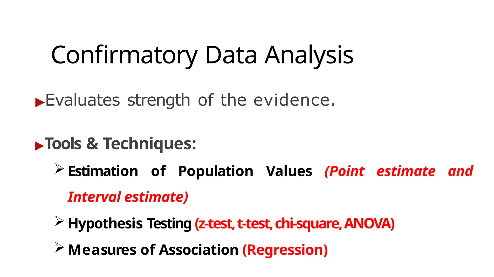
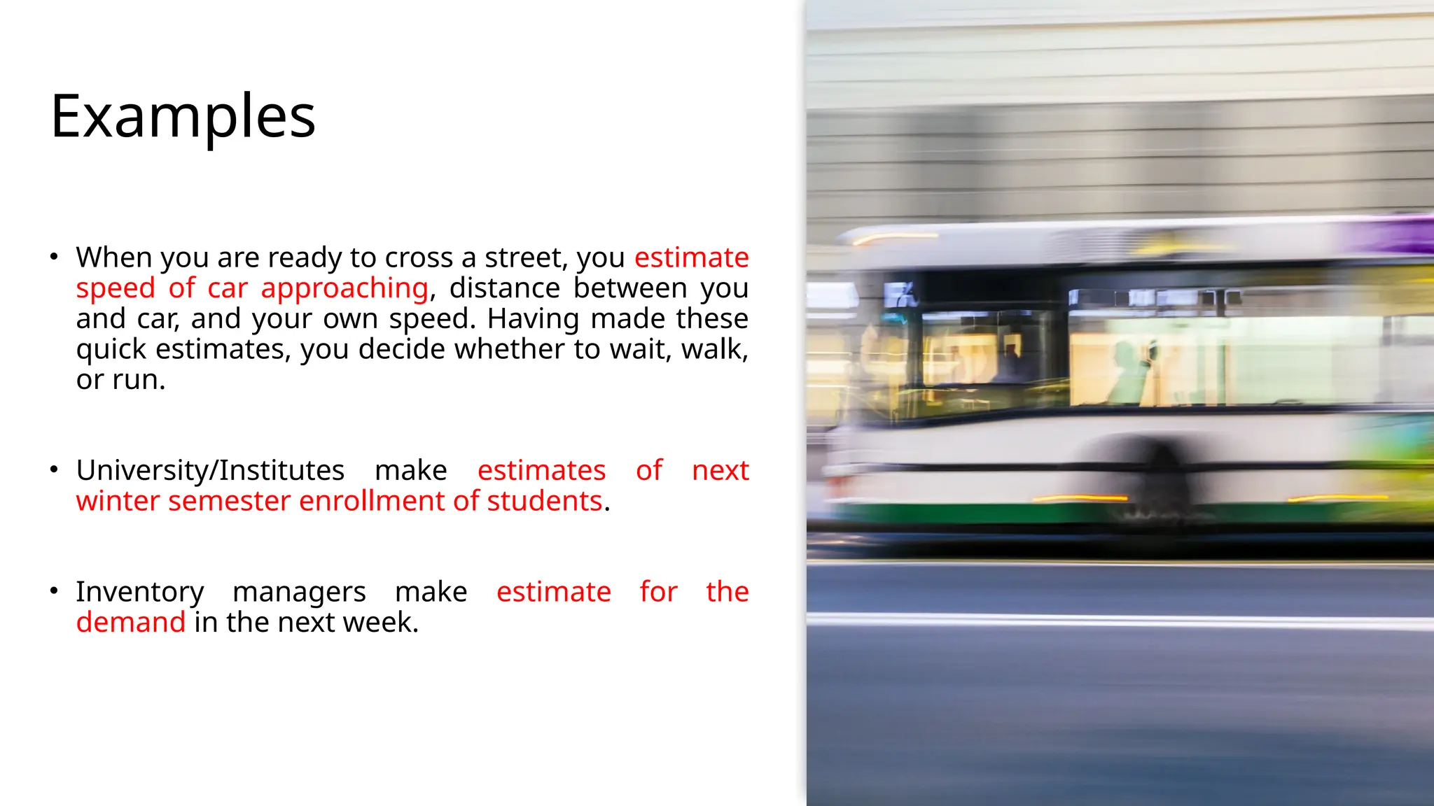
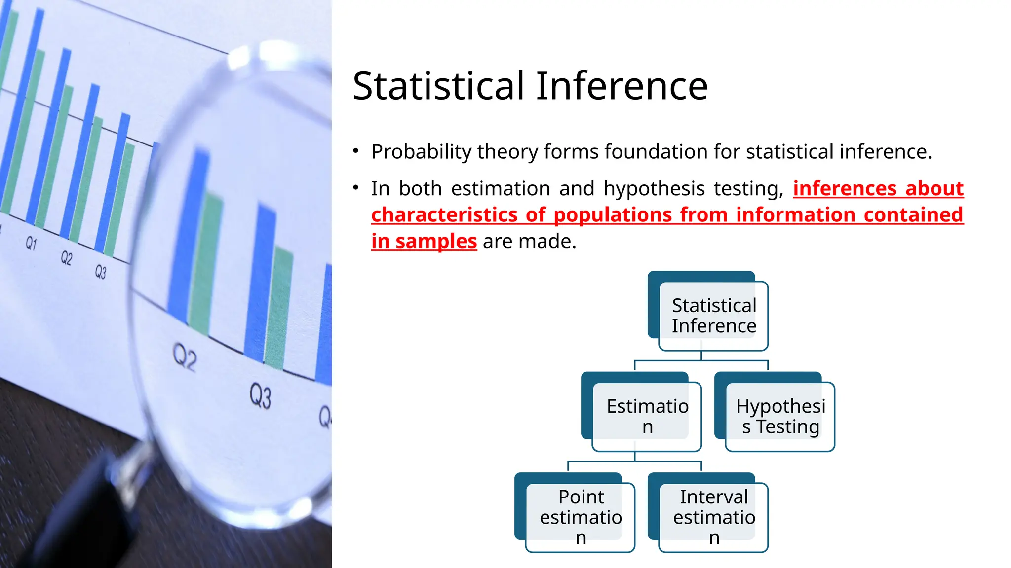
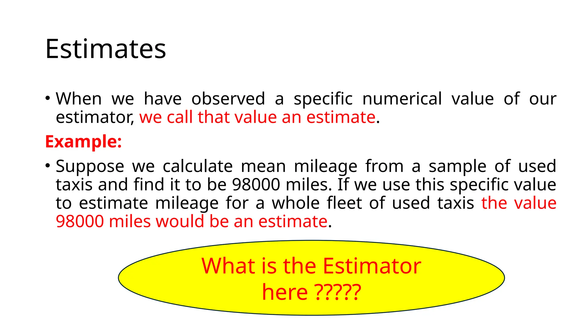
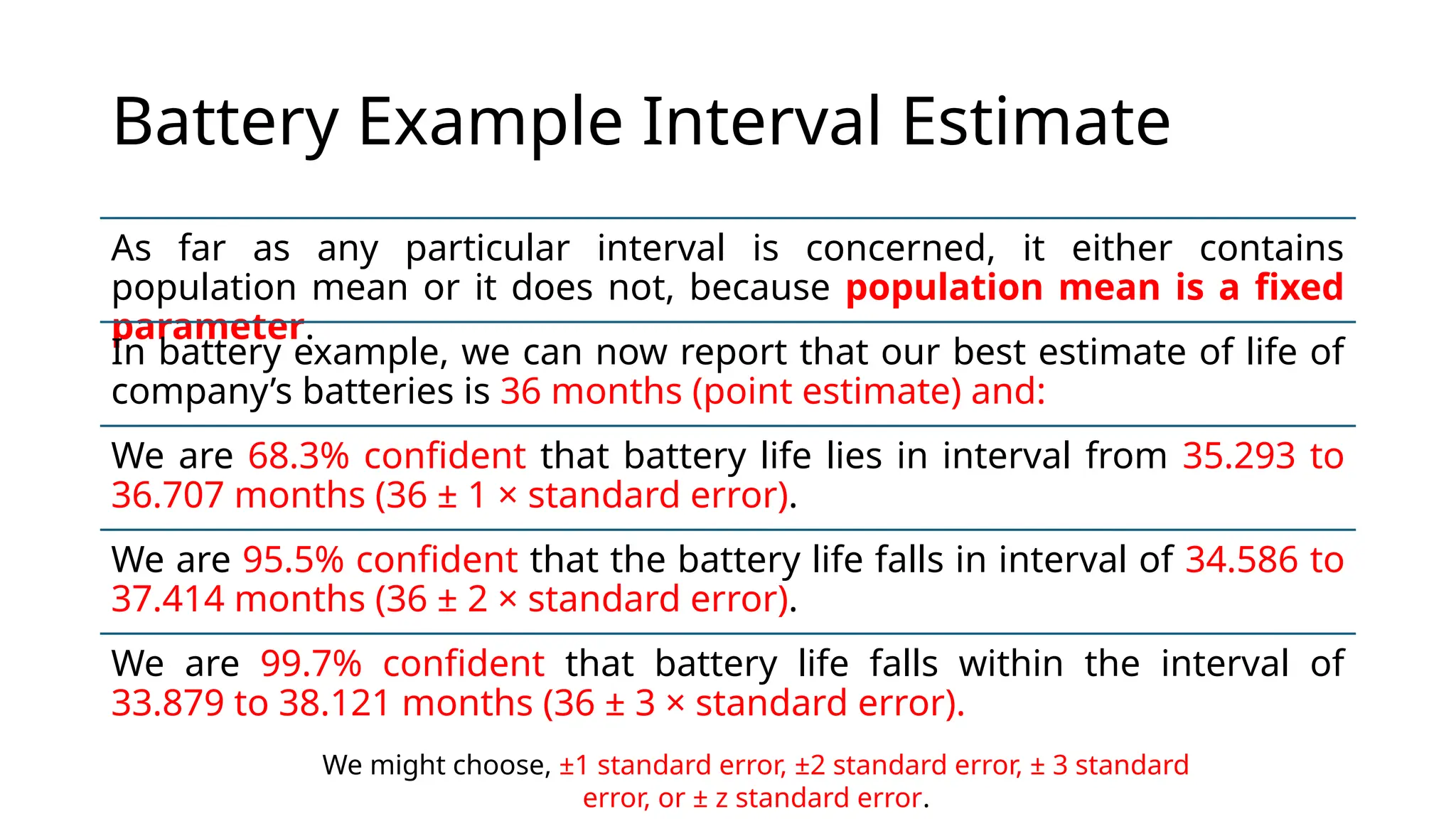
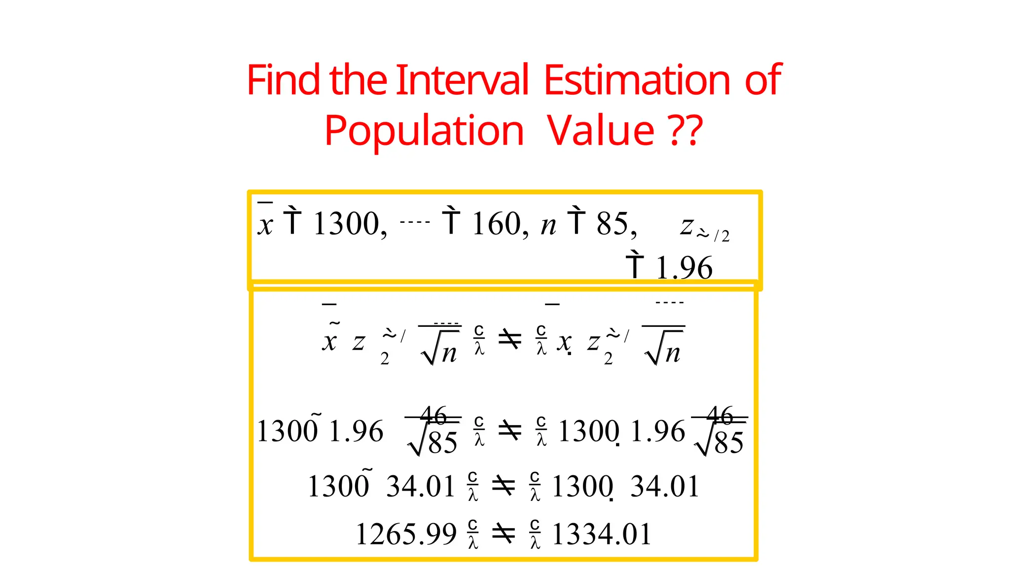
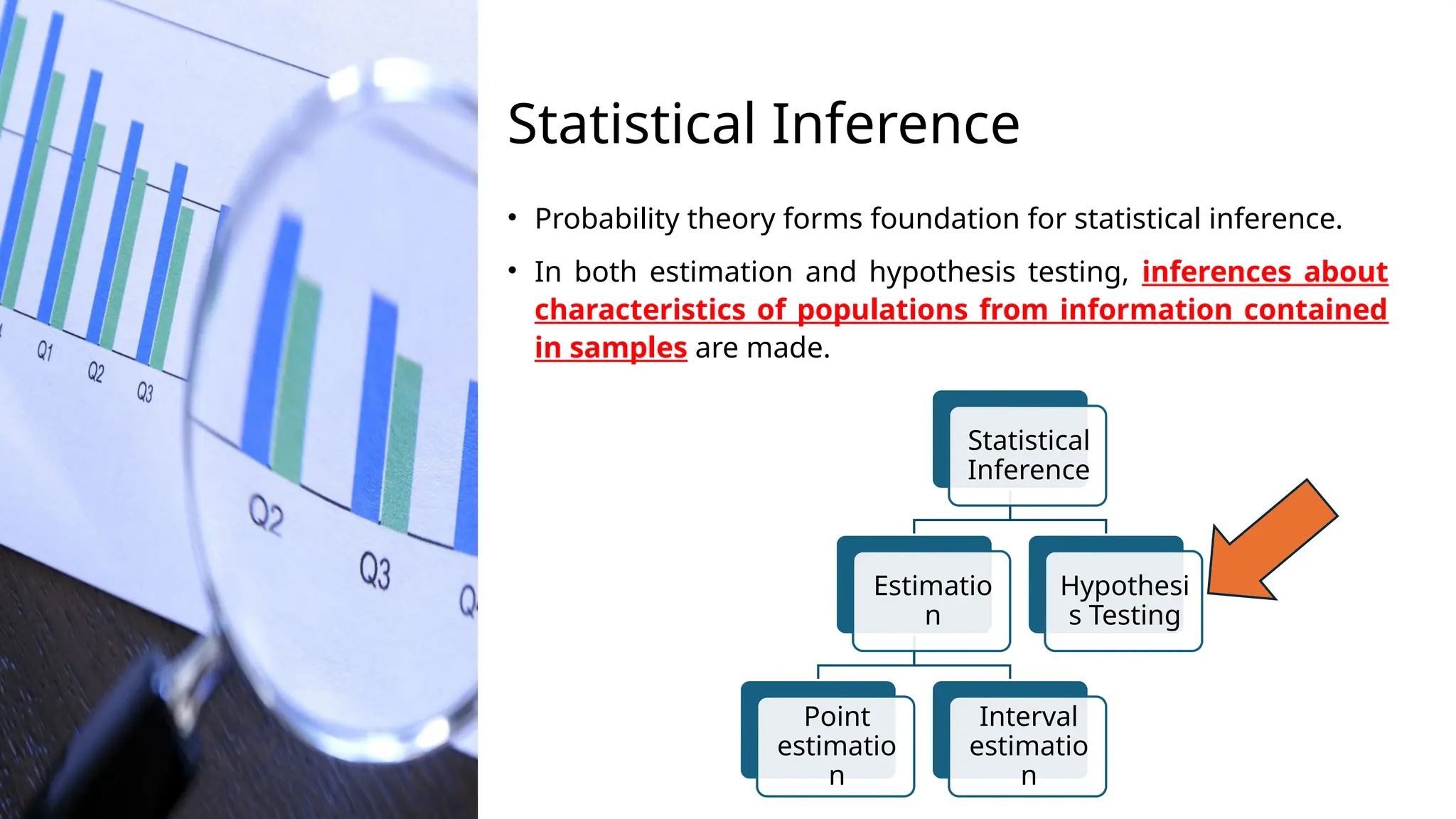
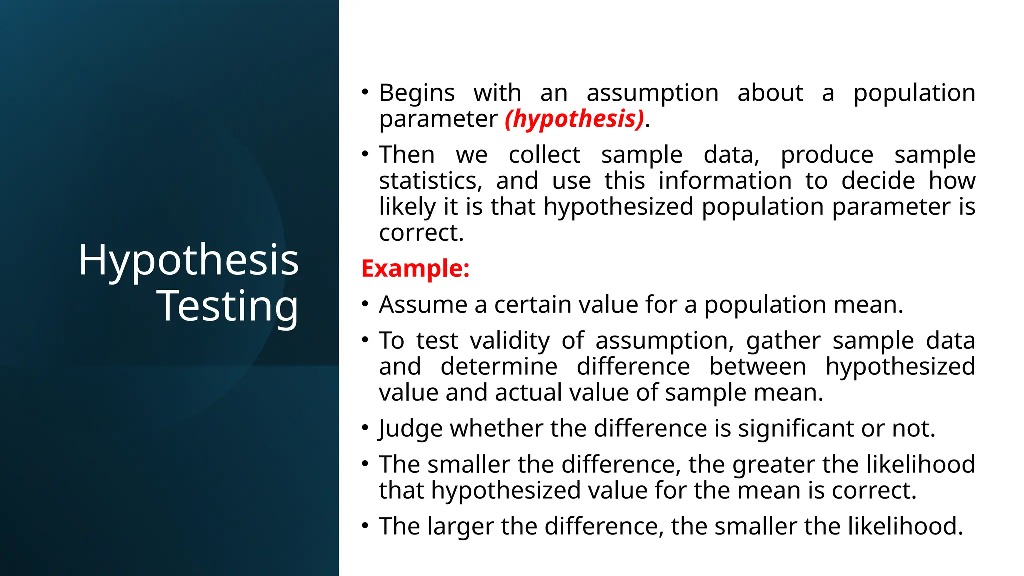
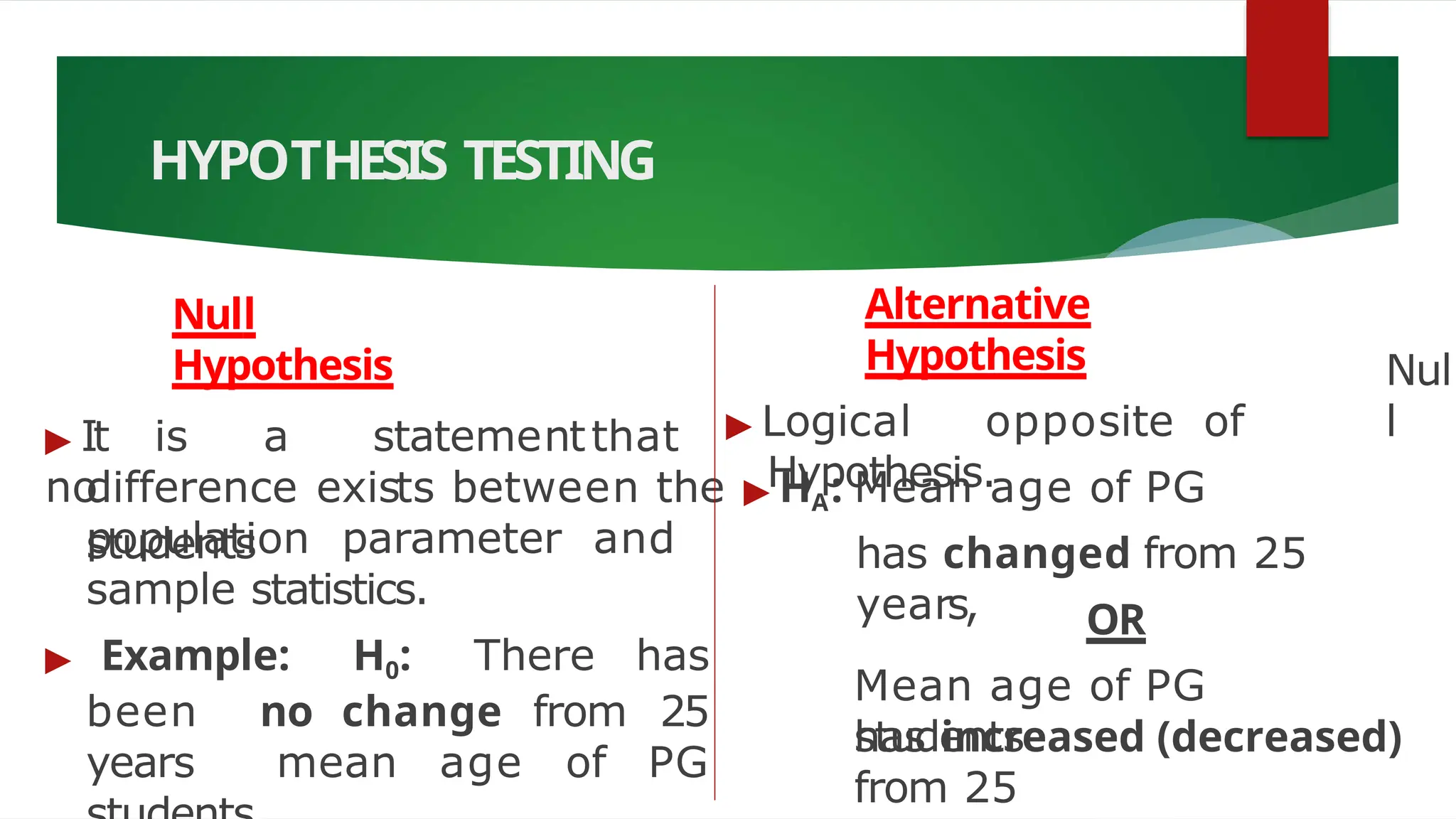
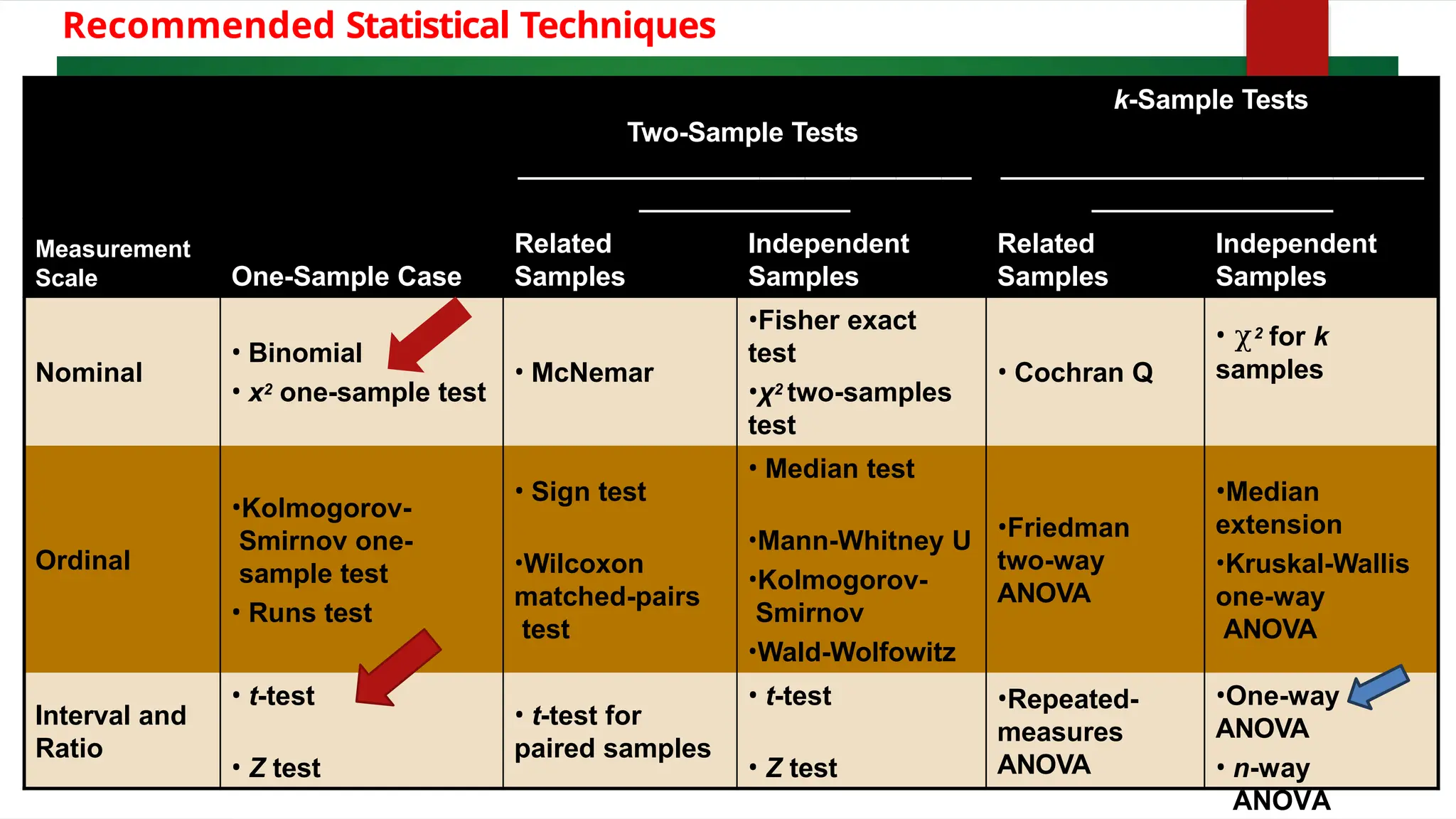
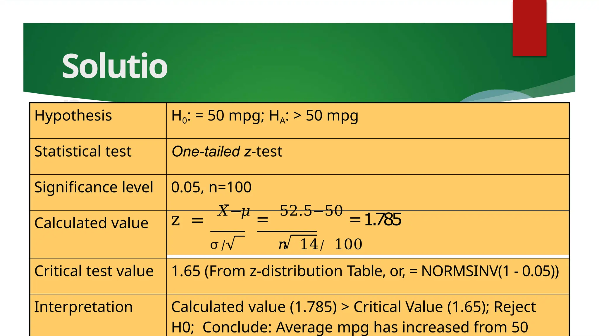
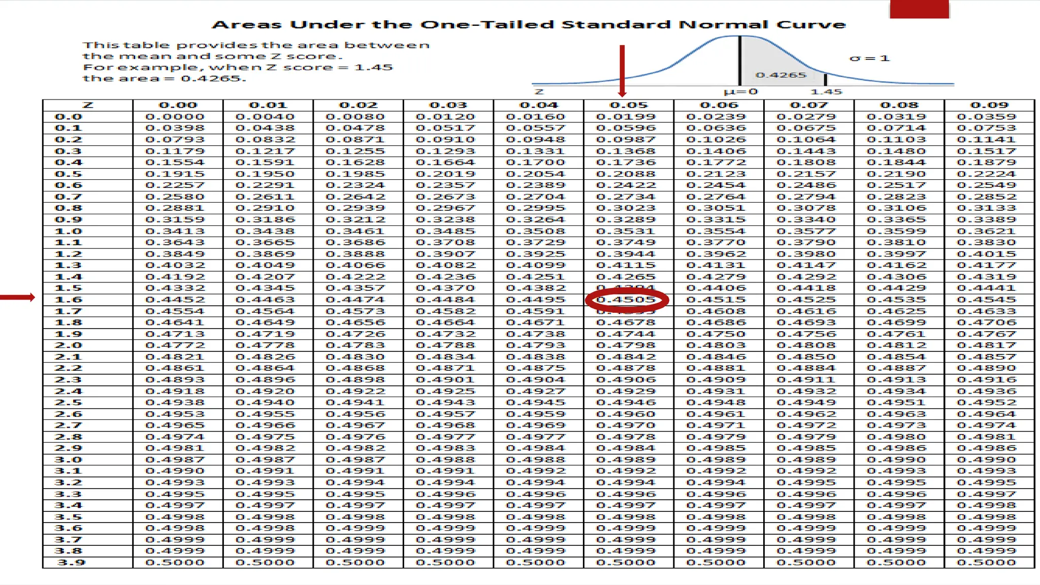
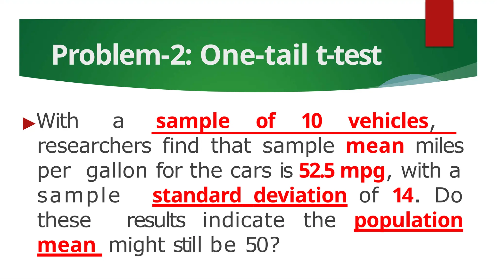
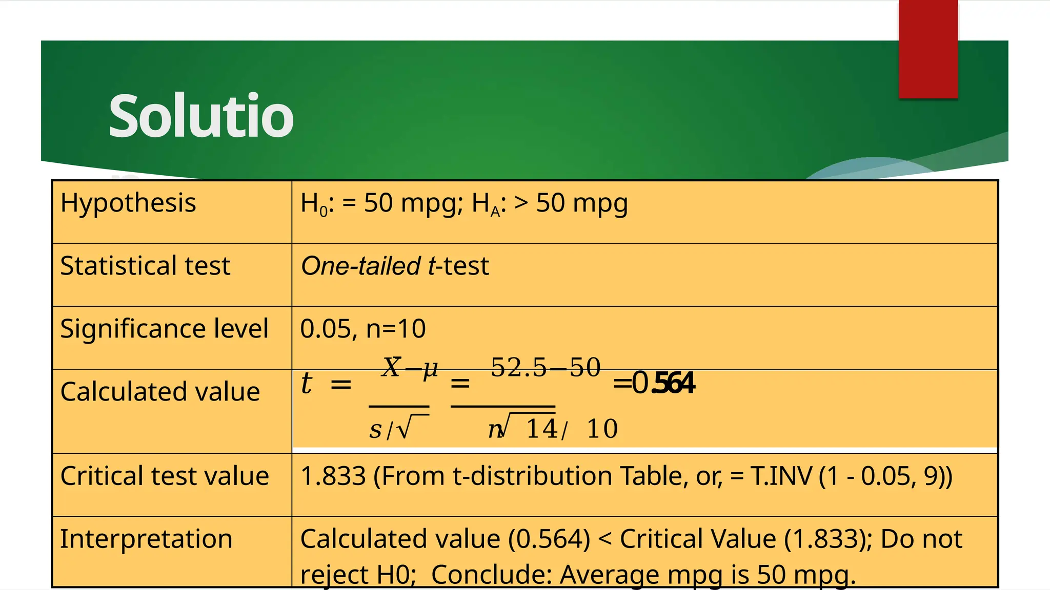
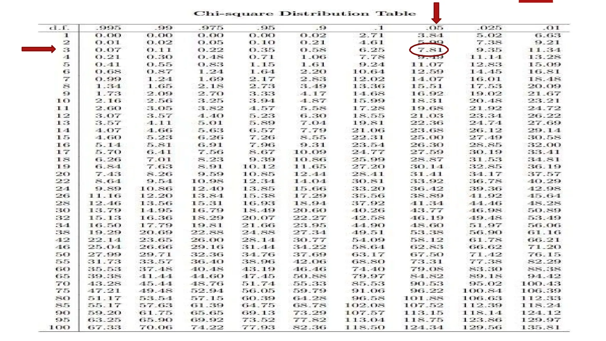
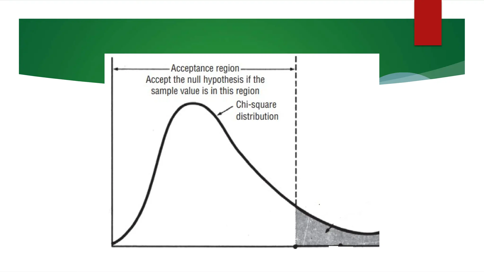
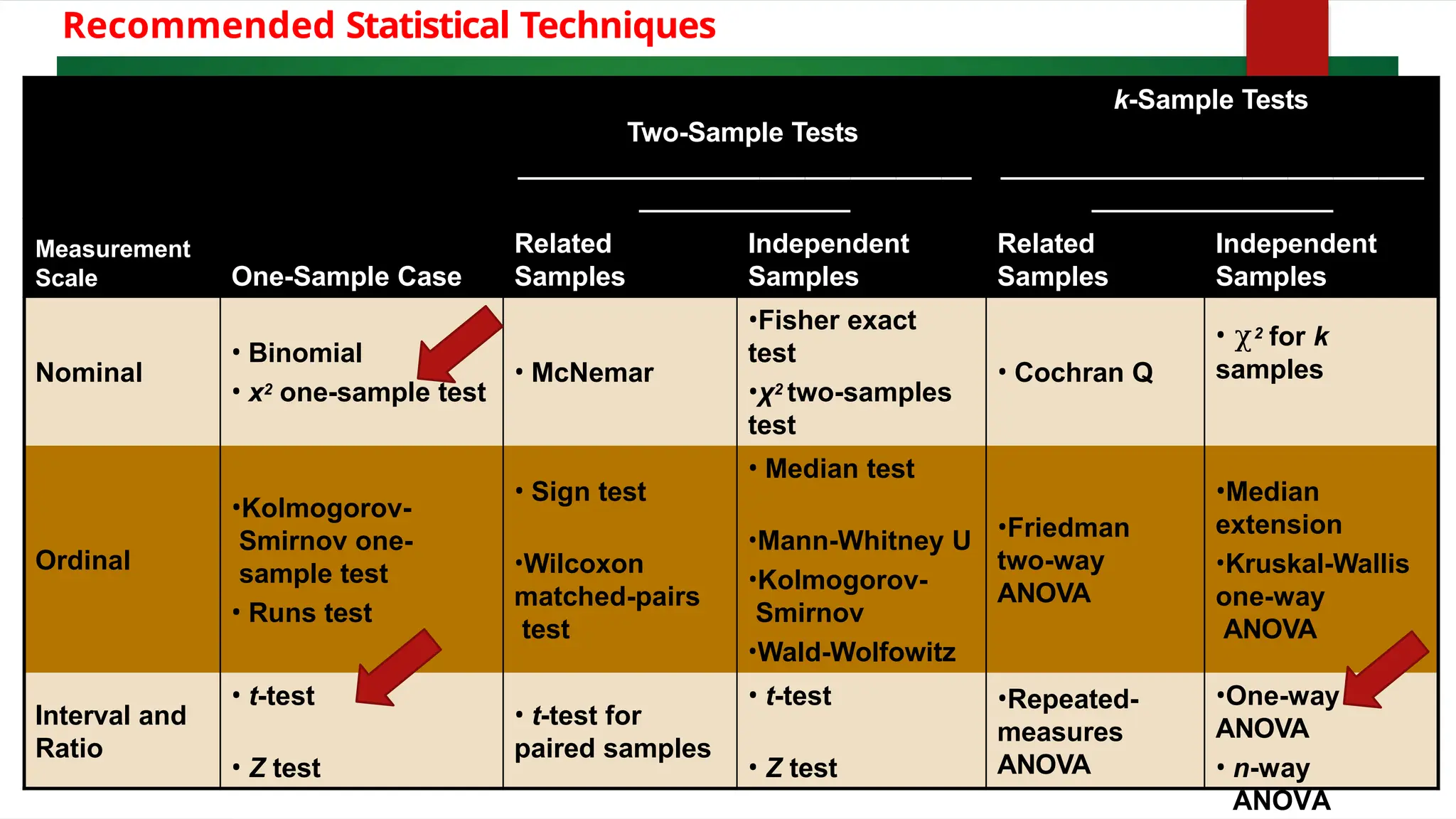
Data Analysis - Confirmatory Data Analysis.pptx

Data Analysis Tools &
Techniques
▶Descriptive Statistics
▶Exploratory Data Analysis (EDA)
▶Confirmatory Data Analysis (CDA)

Confirmatory Data Analysis
▶Evaluates strength of the evidence.
▶Tools & Techniques:
 Estimation of Population Values (Point estimate and
Interval estimate)
 Hypothesis Testing (z-test,t-test,chi-square,ANOVA)
 Measures of Association (Regression)

1. Estimation of
Population Values

Statistical
Estimation
Everyone makes estimates

Examples
• When you are ready to cross a street, you estimate
speed of car approaching, distance between you
and car, and your own speed. Having made these
quick estimates, you decide whether to wait, walk,
or run.
• University/Institutes make estimates of next
winter semester enrollment of students.
• Inventory managers make estimate for the
demand in the next week.

Do you want to make estimates
just by your judgement or by
applying some statistical
techniques ??

Statistical Inference
• Probability theory forms foundation for statistical inference.
• In both estimation and hypothesis testing, inferences about
characteristics of populations from information contained
in samples are made.
Statistical
Inference
Estimatio
n
Point
estimatio
n
Interval
estimatio
n
Hypothesi
s Testing

What is the purpose of gathering samples ?
To learn more about a
population

Estimator
Any sample statistic that is used to
estimate a population parameter is called
an estimator.
Example:
The sample mean can be an estimator of
the population mean.

Estimates
• When we have observed a specific numerical value of our
estimator, we call that value an estimate.
Example:
• Suppose we calculate mean mileage from a sample of used
taxis and find it to be 98000 miles. If we use this specific value
to estimate mileage for a whole fleet of used taxis the value
98000 miles would be an estimate.
What is the Estimator
here ?????

How do managers use
sample statistics to estimate
population parameters?

Types of Estimates about population
• A point estimate is a single number that is used to
estimate an unknown population parameter.
• Example:
A department head would make a point estimate if she said
“Our current data indicate that this course will have 350 students
in the winter semester.”

Point estimators
Point
Estimators
Sample Mean
Sample
Variance and
standard
deviation
Calculate
in Excel
Or,
Which will estimate
population variance??

Is the point estimate sufficient ?
• A point estimate is often insufficient because it is either right or
wrong.
• If you are told only that point estimate of enrollment is wrong, you
do not know how wrong it is, and you cannot be certain of the
estimate’s reliability.
• If you learn that it deviates by only 10 students, you will accept 350
students as a good estimate of future enrollment.
• But if the estimate deviates by 90 students, you will reject it as an
estimate of future enrollment.
• Therefore, a point estimate is much more useful if it is
accompanied by an estimate of the error that might be involved.

Interval Estimates
Interval estimate
describes a range of
values within which a
population parameter
is likely to lie.
• Suppose marketing research director needs
estimate of average battery life of car that his
company manufactures.
• Random sample of 200 battery car owners are
selected.
• Interview conducted with the car owners about
battery life they have experienced.
• Found that Sample of 200 users has mean
battery life of 36 months (point estimate).
• But the director also asks for a statement
about uncertainty that will be likely to
accompany this estimate, i.e., a statement
about the range within which the unknown
population mean is likely to lie.
• To provide such a statement, we need to find
the standard error of the mean.

Standard Error
Suppose we have already estimated the standard deviation of the population of the batteries and
reported that it is 10 months. Using this standard deviation, we can calculate standard error of the
mean:
Actual mean life for all the batteries may lie somewhere
in the interval estimate of 35.293 to 36.707 months.
Next, we need to calculate the chance that the actual life will lie in this
interval or in other intervals of different widths that we might choose,
±2 standard error, ± 3 standard error, or ± z standard error.

• If we select 1,000 samples at random from a given population and then construct an interval of ±2
standard errors around the mean of each of these samples, about 955 of these intervals will include the
population mean.
• Similarly, the probability is 0.683 that the mean of the sample will be within ±1 standard error of the
population mean, and so forth.
Only the interval
constructed around the
sample mean x4-bar does
not contain the population
mean. Statisticians will
describe the interval
estimates as
“The population mean will be
located within ±2 standard errors
from the sample mean 95.5
percent of the time.”
Apply these properties to the
standard error of the mean to
make an interval estimate !!

Battery Example Interval Estimate
As far as any particular interval is concerned, it either contains
population mean or it does not, because population mean is a fixed
parameter.
In battery example, we can now report that our best estimate of life of
company’s batteries is 36 months (point estimate) and:
We are 68.3% confident that battery life lies in interval from 35.293 to
36.707 months (36 ± 1 × standard error).
We are 95.5% confident that the battery life falls in interval of 34.586 to
37.414 months (36 ± 2 × standard error).
We are 99.7% confident that battery life falls within the interval of
33.879 to 38.121 months (36 ± 3 × standard error).
We might choose, ±1 standard error, ±2 standard error, ± 3 standard
error, or ± z standard error.

Z – value Calculation

.4750 .4750
X
95%
.025
.025
Z
1.96
-1.96 0
Example:
For a 95% confidence interval
α = 0.05
α/2 = 0.025
▶ Value of α/2 or z.
0
2
5 look at the
standard normal distribution table
under:
0.5000 - 0.0250 = 0.4750
▶ From standard normal table look up
0.4750 and read 1.96 as the z-value
from the row and column.

x  1300,   160, n  85, z / 2
 1.96
85
n
/
2
/
2

n
x  z

   x  z
1300 1.96
46
   1300 1.96
46
85
1300  34.01    1300  34.01
1265.99    1334.01
FindtheInterval Estimation of
Population Value ??

Hypothesis
Testing
• Begins with an assumption about a population
parameter (hypothesis).
• Then we collect sample data, produce sample
statistics, and use this information to decide how
likely it is that hypothesized population parameter is
correct.
Example:
• Assume a certain value for a population mean.
• To test validity of assumption, gather sample data
and determine difference between hypothesized
value and actual value of sample mean.
• Judge whether the difference is significant or not.
• The smaller the difference, the greater the likelihood
that hypothesized value for the mean is correct.
• The larger the difference, the smaller the likelihood.

We cannot accept or reject a
hypothesis about a population
parameter simply by intuition.
Instead, we need to learn how to
decide objectively, on the basis of
sample information, whether to accept
or reject a hypothesis.

HYPOTHESIS TESTING
Null
Hypothesis
▶ It is a statementthat
no
population parameter and
sample statistics.
▶ Example: H0: There has
been no change from 25
years mean age of PG
Nul
l
Alternative
Hypothesis
▶ Logical opposite of
Hypothesis.
difference exists between the ▶ HA: Mean age of PG
students has changed from 25
years, OR
Mean age of PG
students
has increased (decreased)
from 25

Examples
0
a
H :  >
25
H :  
25
0
a
H :  
25
H :  
25
Which one is One-Tail Test and Which one is Two-Tail
Test of Significance ?????

Tests of Significance
Which one is One-Tail Test and Which one is Two-Tail
Test of Significance ?????

Decision Table for
Hypothesis Testing
Null True Null False
Fail to
reject null
Correct
Decision
Type II error
()
Reject null Type I error
()
Correct
Decision

Rejection and Non-rejection
Regions
Non-Rejection Region

Rejection Region
Critical Value
Rejection Region
Critical Value

▶If the null hypothesis is rejected and
the alternative hypothesis is
accepted, then one can say that a
statistically significant result has been
obtained.
▶With “significant” results, you reject the
null hypothesis.

Types of Tests
Parametric Non-
parametric

How To Select A Test
How many samples are involved?
If two or more samples are involved,
are the individual cases independent or
related?
Is the measurement scale

Recommended Statistical Techniques
Two-Sample Tests
k-Sample Tests
Measurement
Scale One-Sample Case
Related
Samples
Independent
Samples
Related
Samples
Independent
Samples
Nominal
• Binomial
• x2 one-sample test
• McNemar
•Fisher exact
test
•χ2 two-samples
test
• Cochran Q
• χ2 for k
samples
Ordinal
•Kolmogorov-
Smirnov one-
sample test
• Runs test
• Sign test
•Wilcoxon
matched-pairs
test
• Median test
•Mann-Whitney U
•Kolmogorov-
Smirnov
•Wald-Wolfowitz
•Friedman
two-way
ANOVA
•Median
extension
•Kruskal-Wallis
one-way
ANOVA
Interval and
Ratio
• t-test
• Z test
• t-test for
paired samples
• t-test
• Z test
•Repeated-
measures
ANOVA
•One-way
ANOVA
• n-way
ANOVA

CONDITIONS FOR USING THE NORMAL AND
t DISTRIBUTIONS IN TESTING HYPOTHESES
ABOUT MEANS

Statistical Testing Procedures
State
Hypothesis
Choose
Statistical Test
Select Level of
Significance
Compute
difference
Value
Interpret the
Test
Obtain
Critical Test
Value

Problem-1: One-tailed z-test
▶With a sample of 100 vehicles,
researchers find that mean miles per
gallon for the cars is 52.5 mpg. The
population standard deviation is known
to be 14. Do these results indicate the
population mean might still be 50?

Solutio
n
Hypothesis H0: = 50 mpg; HA: > 50 mpg
Statistical test One-tailed z-test
Significance level 0.05, n=100
Calculated value z =
𝑋̅−𝜇
=
52.5−50
=1.785
σ/ 𝑛 14/ 100
Critical test value 1.65 (From z-distribution Table, or, = NORMSINV(1 - 0.05))
Interpretation Calculated value (1.785) > Critical Value (1.65); Reject
H0; Conclude: Average mpg has increased from 50

Problem-2: One-tail t-test
▶With a sample of 10 vehicles,
researchers find that sample mean miles
per gallon for the cars is 52.5 mpg, with a
sample standard deviation of 14. Do
these results indicate the population
mean might still be 50?

Solutio
n
Hypothesis H0: = 50 mpg; HA: > 50 mpg
Statistical test One-tailed t-test
Significance level 0.05, n=10
Calculated value 𝑡 =
𝑋̅−𝜇
=
52.5−50
=0.564
𝑠/ 𝑛 14/ 10
Critical test value 1.833 (From t-distribution Table, or, = T.INV (1 - 0.05, 9))
Interpretation Calculated value (0.564) < Critical Value (1.833); Do not
reject H0; Conclude: Average mpg is 50 mpg.

Problem-3
▶We interviewed 200 students and learned their
intentions to join the University club. We would
like to analyse the results by living
arrangement. The 200 responses are classified
into the four categories given in the Table.

Living
Arrangement
Intend to
Join
(Observed, O)
Number
Interviewed
Percent
(no.
interviewed/
200)
Expected
Frequencies (E)
(percent x 60)
Dorm 16 90 45% 27
Apartment/
House nearby
13 40 20% 12
Apartment/
House distant
16 40 20% 12
Live at home 15 30 15% 9
Total 60 200 100 60

Solutio
n
Null H0: Joining club and Living arrangement are independent
Ha: Joining club depends on Living arrangement
Statistical test One-sample chi-square non-parametric
test
Significance 0.05
level
Calculate
d value
𝑖
χ 2 = 𝑖 𝑖
=
2 2
𝑂 − 𝐸16 − 27 13 − 12 2
16 −
12
2
+ + +
15 −
9
2
𝐸𝑖 27 12 12 9
=
9.89
Degrees of freedom = (No. of Categories – 1) = (4 - 1) = 3
Critical
test
value
7.81 (from Chi-square Statistical Table or, = CHISQ.INV(1-0.05,3))
Interpretati
on
Calculated Value (9.89) > Critical Value (7.81) so Reject H0.
Conclude: Intending to join club is dependent on living
arrangement.

Data Analysis - Confirmatory Data Analysis.pptx

More Related Content

Similar to Data Analysis - Confirmatory Data Analysis.pptx

Recently uploaded

Data Analysis - Confirmatory Data Analysis.pptx

Editor's Notes