Downloaded 341 times


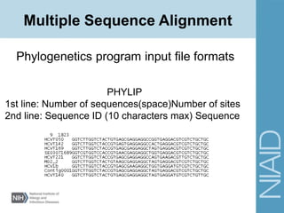
![NEXUS
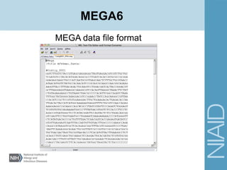
#NEXUS
[Name: HCVT050 Len: 1823 Check: 5A341084]
[Name: HCVT142 Len: 1823 Check: AB5C0B76]
[Name: HCVT169 Len: 1823 Check: 7EAF66DA]
[Name: SE03071689 Len: 1823 Check: 1EFF8405]
[Name: HCVT221 Len: 1823 Check: 3D0C96F0]
[Name: MD2_2 Len: 1823 Check: 1E2A0948]
[Name: HCV1b Len: 1823 Check: BC29D7FB]
[Name: Contig0001 Len: 1823 Check: CD240524]
[Name: HCVT140 Len: 1823 Check: 2A5C0D4E]
begin data;
dimensions ntax=9 nchar=1823;
format datatype=dna interleave missing=-;
matrix
HCVT050 GGTCTTGGTCTACTGTGAGC GAGGAGGCCGGTGAGGACGT
HCVT142 GGTCTTGGTCTACCGTGAGT GAGGAGGCCACTGAGGACGT
HCVT169 GGTCTTGGTCTACCGTGAGC GAGGAGGCTAGTGAGGACGT
SE0307168 GGTCGTGGTCCACCGTGAAC GAGGAGGCTGGTGAGGACGT
HCVT221 GGTCTTGGTCTACCGTGAGC GAGGAGGCCAGTGAAGACGT
MD2_2 GGTCTTGGTCTACTGTAAGC GAGGAGGCTAGTGAGGACGT
HCV1b GGTCTTGGTCTACCGTGAGC GAAGAGGCTGGTGAGGATGT
Contig000 GGTCTTGGTCTACCGTGAGC GAGGAGGCTAGTGAGGACGT
HCVT140 GGTCTTGGTCTACTGTGAGC GAGGAGGCTAGTGAGGATGT
;
end;
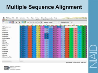
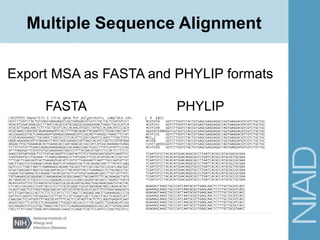
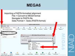
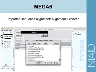
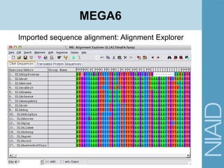
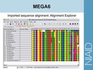
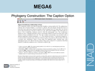
Phylogenetics program input file formats
Multiple Sequence Alignment](https://image.slidesharecdn.com/lecture3fall2015-170302022555/85/Phylogenetics-Tree-building-34-320.jpg)
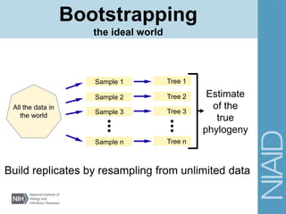
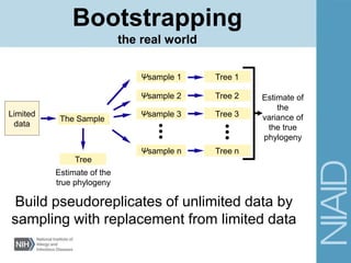
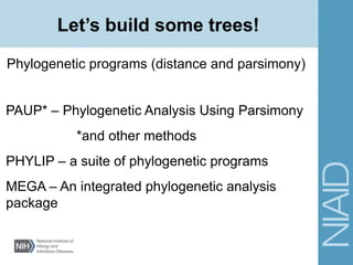


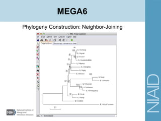
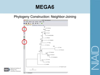
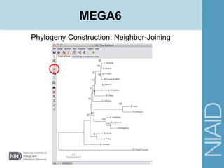


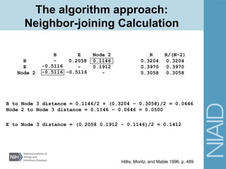
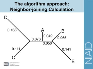
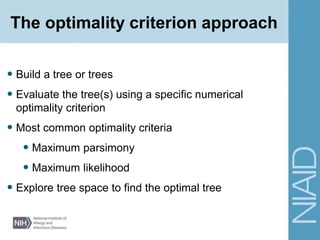
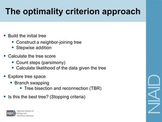
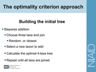
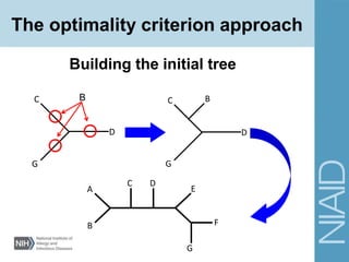
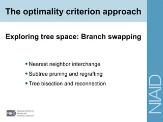
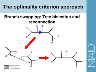
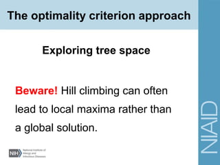
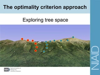
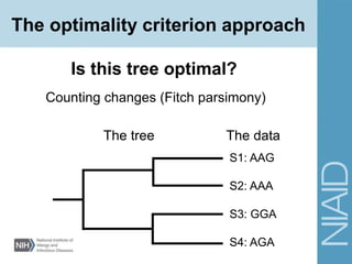
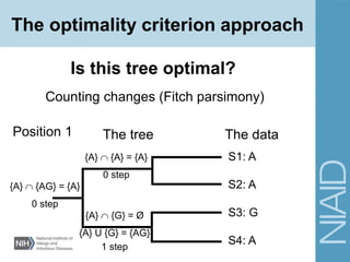
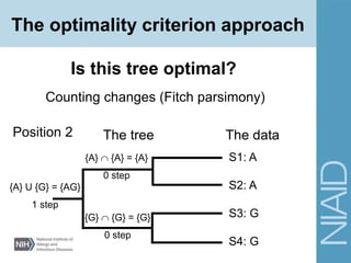
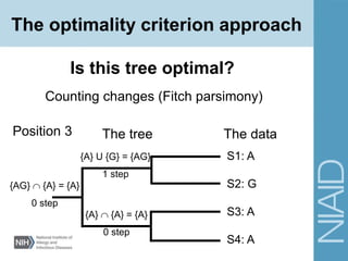
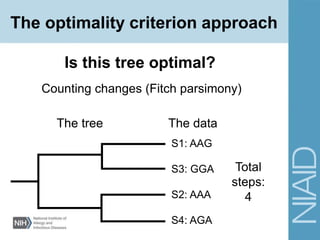
This document provides an overview of phylogenetic analysis concepts and methods. It begins with an introduction to phylogenetic trees and their components. It then covers two main approaches to building trees - using distance methods like neighbor-joining and using optimality criteria like maximum parsimony. Key steps in both approaches like multiple sequence alignment and tree-building algorithms are described. The document concludes with discussing tools for evaluating tree reliability through bootstrapping and exploring available phylogenetics programs.