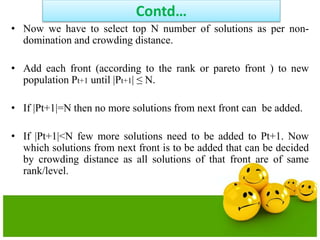
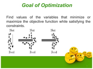
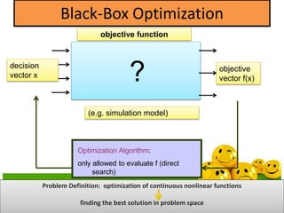
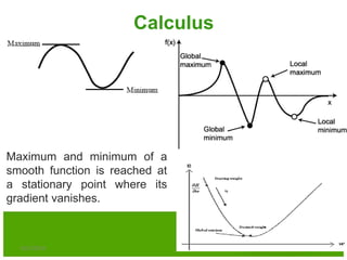
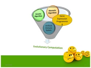
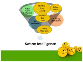
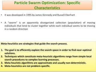
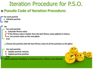
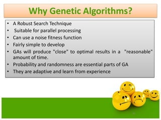
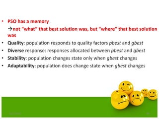
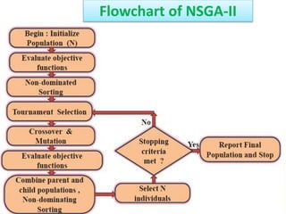
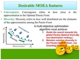
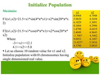
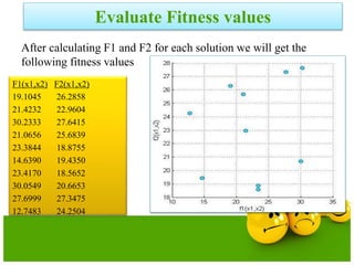
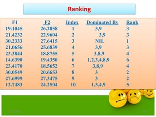
The document discusses various optimization techniques including evolutionary computing techniques such as particle swarm optimization and genetic algorithms. It provides an overview of the goal of optimization problems and discusses black-box optimization approaches. Evolutionary algorithms and swarm intelligence techniques that are inspired by nature are also introduced. The document then focuses on particle swarm optimization, providing details on the concepts, mathematical equations, components and steps involved in PSO. It also discusses genetic algorithms at a high level.

1. Optimization Using
Evolutionary Computing
Techniques
Prof. (Dr.) Pravat Kumar Rout
Department of EEE, ITER
Siksha ‘O’ Anusandhan (Deemed to be
University),
Bhubaneswar, Odisha, India

2. Goal of Optimization
Find values of the variables that minimize or
maximize the objective function while satisfying the
constraints.
2

3. ?
Black-Box Optimization
Optimization Algorithm:
only allowed to evaluate f (direct
search)
decision
vector x
objective
vector f(x)
objective function
(e.g. simulation model)
Problem Definition: optimization of continuous nonlinear functions
finding the best solution in problem space

4. Calculus
Maximum and minimum of a
smooth function is reached at
a stationary point where its
gradient vanishes.
6/21/2013 4

5. 6/21/2013 5
Why Evolutionary Computation
Exact Mathematical Expression (Not being applicable to
certain class of objective functions in case of classical
techniques)
 Derivative Free
Global Optimization(Not trapped at local minima in case
of classical technique)
Less Computational Complexity

6. Other class of Heuristics
Inspired By Nature
 Evolutionary Algorithms (EA)
– All methods inspired by the evolution
 Swarm Intelligence (SI)
– All methods inspired by collective intelligence
 Geographical Nature Algorithm (GNA)
– All methods inspired by geographical structure of the
environment/ earth
66/21/2013

7. 6/21/2013 7
Gene
Expression
Programmin
g

8. 6/21/2013 8
Swarm Intelligence
Bat
Optimization
Particle
Swarm
Intelligence
Ant Colony
Optimization
Firefly
Algorithm
Cukoo
Search
Shuffled
Frog
Leaping
Artificial
Bee
Colony

9. 6/21/2013 9
Geographical Nature Optimization
River
Formation
Dynamics
Bio-geographical
Optimization
Weed
Optimization

10. Other Types of Search Techniques
6/21/2013 10
Differential
Evolution
Seeker
Optimization
Hybrid
Techniques
HARMONY
Search

11. Component of Optimization Problem
• Objective Function: An objective function which we want to
minimize or maximize.
• In clustering problem to fix the cluster center such that
maximize inter cluster distance and minimize intra cluster
distance.
• For example, in a manufacturing process, we might want to
maximize the profit or minimize the cost.
• In fitting experimental data to a user-defined model, we might
minimize the total deviation of observed data from predictions
based on the model.
• In designing an inductor, we might want to maximize the Quality
Factor and minimize the area.
6/21/2013 11

12. Component of Optimization Problem
• Design Variables: A set of unknowns or variables which affect
the value of the objective function.
• In clustering problem it may be the number of features which
define the center of the cluster
• In the manufacturing problem, the variables might include the
amounts of different resources used or the time spent on each
activity.
• In fitting-the-data problem, the unknowns are the parameters
that define the model.
• In the inductor design problem, the variables used define the
layout geometry of the panel.
6/21/2013 12

13. Component of Optimization Problem
• Constraints: A set of constraints that allow the unknowns to take
on certain values but exclude others.
• The limits of the features value in the clustering problem
• For the manufacturing problem, it does not make sense to spend a
negative amount of time on any activity, so we constrain all the
"time" variables to be non-negative.
• In the inductor design problem, we would probably want to limit
the upper and lower value of layout parameters and to target an
inductance value within the tolerance level.
6/21/2013 13

14. Mathematical Formulation of
Optimization Problems
 
 
1 2
minimizetheobjectivefunction
min ( ), , ,.......,
subject toconstraints
( ) 0
0
n
i
i
f x x x x x
c x
c x



   
2 2
1 2
2 2
1 2
1 2
Example
min 2 1
subject: 0
2
x x
x x
x x
   
 
 
 
6/21/2013 14
Inequality constraints: x1
2 – x2
2 < 0
Equality constraints: x1 = 2

15. 6/21/2013 15
How can birds or fish exhibit
such a coordinated
collective behavior?
Origin of PSO
Concept:
based on bird
flocks and fish
schools
Swarm: a large or dense group
of flying insects.

16. 6/21/2013 16
•In PSO, each single solution is a "bird" in the search space. Call it
"particle".
•All of particles have fitness values
•which are evaluated by the fitness function to be optimized, and
•have velocities
•which direct the flying of the particles.
•The particles fly through the problem space by following the current
optimum particles.
What is PSO?

17. Particle Swarm Optimization: Specific
Characteristics
• It was developed in 1995 by James Kennedy and Russell Eberhart
• A “swarm” is an apparently disorganized collection (population) of moving
individuals that tend to cluster together while each individual seems to be moving
in a random direction
6/21/2013 17
Meta-heuristics are strategies that guide the search process.
1. The goal is to efficiently explore the search space in order to find near–optimal
solutions.
2. Techniques which constitute meta-heuristic algorithms range from simple local
search procedures to complex learning processes.
3. Meta-heuristic algorithms are approximate and usually non-deterministic.
4. Meta-heuristics are not problem-specific.

18. Continued…
• It uses a number of agents (particles) that constitute a swarm moving
around in the search space looking for the best solution (based on
bird flocks and fish schools).
• Each particle is treated as a point in a D-dimensional space which
adjusts its “flying” according to its own flying experience as well as
the flying experience of other particles
• Each particle keeps track of its coordinates in the problem space
which are associated with the best solution (fitness) that has
achieved so far. This value is called pbest.
• Another best value that is tracked by the PSO is the best value
obtained so far by any particle in the neighbors of the particle. This
value is called gbest.
• The PSO concept consists of changing the velocity(or accelerating) of
each particle toward its pbest and the gbest position at each time
step.
6/21/2013 18

19. PSO Basic Mathematical Equations
pi
vt
xt pg
xt+1
   1 1 2 , 3 ,
1 1
t t i t t g t t
t t t
v c v c p x c p x
x x v

 
     

 
,
,
1 2 3
: velocity at time step
: position at time step
: best previous position, at time step
: best previous best, at time step ,
, , : co
neighbour'
gnitive/social
s
t
t
i t
g t
v t
x t
p t
p t
c c c




 confidence coefficients
where
particle’s itself
particle’s personal best
particle’s neighbours best
Inertia
Factor
Personal
Influence
Factor
Social Influence Factor

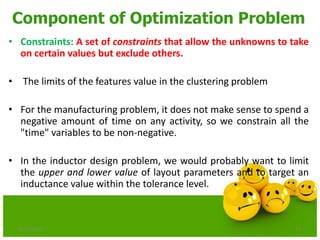
20. 20
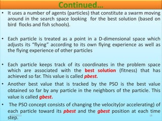
PSO Velocity Update Equations Using
Constriction Factor Method
0.729)Kso4.1,set towas(
4,
42
2
)]()([
21
2
2211









cc
K
vxx
xprandcxprandcvKv
new
id
old
id
new
id
idgdidid
old
id
new
id

21. PSO algorithm
Initialize particles with random
position and zero velocity
Evaluate fitness value
Compare & update fitness value
with pbest and gbest
Meet stopping
criterion?
Update velocity and
position
Start
End
YES
NO
pbest = the best
solution (fitness)
a particle has
achieved so far.
gbest = the global
best solution of
all particles.

22.  Pseudo Code of Iteration Procedure:
For each particle
Initialize particle
END
Do
For each particle
Calculate fitness value
If the fitness value is better than the best fitness value (pBest) in history
set current value as the new pBest
End
Choose the particle with the best fitness value of all the particles as the gBest
For each particle
Update particle velocity
Update particle position
End
While maximum iterations or minimum error criteria is not attained
Iteration Procedure for P.S.O.

23. Advantages Over Other Optimization Technique
• It is derivative free technique unlike many conventional technique
• It has the flexibility to integrated with other optimization techniques to form
hybrid tools
• It is less sensitive to the nature of the objective function that is convexity or
continuity
• It has less parameters to adjust unlike many other competing evolutionary
techniques
• It has the ability to escape the local minima
• It is easy to implement and program with basic mathematical and logic
operations
• It does not require a good initial solution to start its iteration process
• It can handle objective functions with stochastic nature, like in the case of
representing one of the optimization variables as random
6/21/2013 23

24. Disadvantages of PSO
• Lack of solid mathematical background
• failure to assure global optimal solution
• the social influence aspect of the algorithm
• generalized rules in how to tune its parameters to suit
different optimization problems
• coefficient adjustment not clear methodology
6/21/2013 24

25. Schwefel's function
n:1=i420.9687,=
418.9829;=)(
minimumglobal
500500
where
)sin()()(
1



 
i
i
n
i
ii
x
nxf
x
xxxf
6/21/2013 25

26. DECLARATION OF VARIABLES AND THEIR
MEANING
% itermax: Maximum Iteration Number
% c1, c2 : Two parameters for PSO algorithm
% wmax, wmin : these are the maximum and minimum value
of the parameter w
% population_size: Size of the population/number of particles
% var_max : maximum value of the variable
% var_min : minimum value of the variable
% var_size : total number of variables
% population: matrix of value of all the particles/ solutions
6/21/2013 26

27. % pbest: personal best value
% pbest_value: personal best fitness value
% gbest: group best among all particles
% gbest_value: fitness value of the best among the
group
% velocity_max = maximum value of the velocity
% velocity_min = minimum value of the velocity
6/21/2013 27

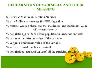
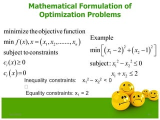
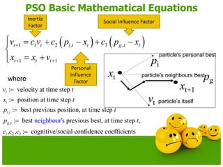
28. Step-1: INITIALIZATION OF VARIABLES
itermax = 100;
c1 = 2;
c2 = 2;
wmax = 0.9;
wmin = 0.4;
population_size = 20;
var_max = [5.12 5.12];
var_min = [-5.12 -5.12];
velocity_max = var_max;
velocity_min = var_min;
var_size =
length(var_max);
6/21/2013 28

29. Step-2:Initial Position
population = zeros(population_size, var_size);
velocity = zeros(population_size, var_size);
velocity_new = zeros(population_size, var_size);
for i = 1:population_size
for j = 1:var_size
population(i,j) = var_min(1,j) + rand*(var_max(1,j) -
var_min(1,j));
end
end
6/21/2013 29

30. for i = 1:population_size
for j = 1:var_size
velocity(i,j) = velocity_min(1,j) +
rand*(velocity_max(1,j) -
velocity_min(1,j));
end
end
Step-3:Initial Velocity
6/21/2013 30

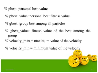
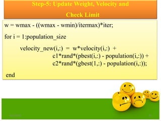
31. fitness = objective_function(population);
pbest = population;
pbest_value = fitness;
[ xx yy] = min(fitness);
gbest = population(yy,:);
gbest_value = xx ;
Step-4:Determination of Pbest & Gbest
6/21/2013 31

32. Loop
for iter = 1:itermax
Step-5: Update Weight, Velocity and Check limit
Step-6: Update Position & Limit Checking
Step-7:Modifying Pbest & Gbest
Step-8: Graph & Data Presentation
end
6/21/2013 32

33. w = wmax - ((wmax - wmin)/itermax)*iter;
for i = 1:population_size
velocity_new(i,:) = w*velocity(i,:) +
c1*rand*(pbest(i,:) - population(i,:)) +
c2*rand*(gbest(1,:) - population(i,:));
end
Step-5: Update Weight, Velocity and
Check Limit
6/21/2013 33

34. Contd. …
for i = 1:population_size
for j = 1:var_size
if velocity_new(i,j) > velocity_max(j)
velocity_new(i,j) = velocity_max(j);
elseif velocity_new(i,j) < velocity_min(j)
velocity_new(i,j) = velocity_min(j);
end
end
end
6/21/2013 34

35. population_new = population + velocity_new;
for i = 1:population_size
for j = 1:var_size
if population_new(i,j) > var_max(j)
population_new(i,j) = var_max(j);
elseif population_new(i,j) < var_min(j)
population_new(i,j) = var_min(j);
end
end
end
Step-6: Update Position & Check Limit
6/21/2013 35

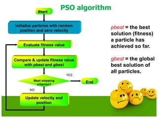
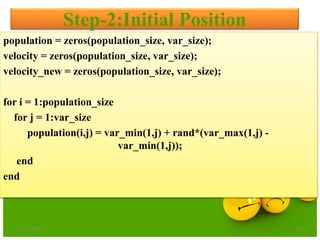
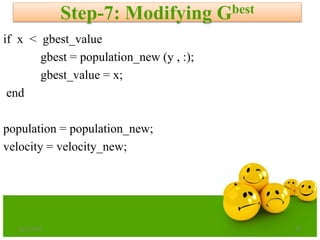
36. Step-7: Modifying Pbest
fitness_new = objective_function(population_new);
[ x y] = min(fitness_new);
for i = 1:population_size
if fitness_new(i)< pbest_value
pbest(i,:) = population_new(i,:);
pbest_value(i) = fitness_new(i);
end
end
6/21/2013 36

37. if x < gbest_value
gbest = population_new (y , :);
gbest_value = x;
end
population = population_new;
velocity = velocity_new;
Step-7: Modifying Gbest
6/21/2013 37

38. Step-8: Graphs & Data Presentation
best_value(iter) = gbest_value;
drawnow
plot(best_value);
6/21/2013 38

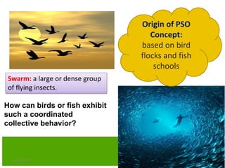
39. Objective Function
function fitness = objective_function(population)
[row_population col_population] = size(population);
for i = 1: row_population
for j = 1: col_population
xx(j) = population(i,j);
end
fitness(i) = 20 + xx(1)^2 + xx(2)^2 -
10*(cos(2*pi*xx(1))+cos(2*pi*xx(2)));
end
6/21/2013 39

40. 40
What is Genetic Algorithms?
• Inverted by Prof. John Holland at the university of Michigan in 1975
• A genetic algorithm (or short GA) is a search technique used in
computing to find true or approximate solutions to optimization and
search problems.
• It uses two basic processes from evolution: “inheritance”(passing of
features from one generation to next) and competition ,“survival of
the fittest” (weeding out the bad features from individuals in the
populations).

41. 41
Why Genetic Algorithms?
• A Robust Search Technique
• Suitable for parallel processing
• Can use a noise fitness function
• Fairly simple to develop
• GAs will produce "close" to optimal results in a "reasonable"
amount of time.
• Probability and randomness are essential parts of GA
• They are adaptive and learn from experience

43. 43
Pseudo-code algorithm
of Genetic Algorithm
1:Choose initial population
2: Evaluate the fitness of each individual in the population
3:Repeat
1: Select best-ranking individuals to reproduce
2: Breed new generation through crossover and
mutation (genetic operations) and give birth
to offspring
3: Evaluate the individual fatnesses of the offspring
4: Replace worst ranked part of population with
offspring
4:Until <terminating condition>

44. Problem
6/21/2013 44
Maximize
F(x1, x2) = 21.5 + x1*sin(4* *x1)
+ x2*sin(20* *x2);
Where –3.0 x1 12.1
and 4.1 x2 5.8

45. 45
Continue: Problem
• If the optimization problem is to minimize a
function f, this is equivalent to maximizing a
function g, where g = -f e.g
min f(x) = max g(x) = max {-f(x)}
or
min f(x) = max g(x) = max (1/f(x))

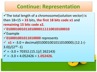
46. Step:1 Representation
6/21/2013 46
Assume the required precision for each variable is upto
four decimal places.
The variable x1 has length 15.1 e.g [12.1 –3.0]
 The precision requirement implies that the range[-3.0,
12.1] should be divided into at least 15.1*10000 equal size
ranges.
This means that 18 bits are required for the first part of the
chromosome.
 217< 151000 <218

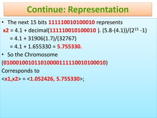
47. 47
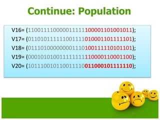
Continue: Representation
• The domain of variable x2 has length 1.7 e.g.[5.8-4.1]
• The precision requirement implies that the range [4.1,
5.8] should be divided into at least 1.7*10000 equal size
ranges.
• This means that 15 bits are required as the second part
of the chromosome.
214< 17000 <215

48. Continue: Representation
6/21/2013 48
The total length of a chromosome(solution vector) is
then 18+15 = 33 bits, the first 18 bits code x1 and
remaining 15 bits code x2.
010001001011010000111110010100010
Example
010001001011010000 represents
 x1 = -3.0 + decimal(010001001011010000).(12.1-(-
3.0))/(218 -1)
 = -3.0 + 70352.(15.1)/( 262143)
 = -3.0 + 4.052426 = 1.052426.

49. 49
Continue: Representation
• The next 15 bits 111110010100010 represents
x2 = 4.1 + decimal(111110010100010 ). (5.8-(4.1))/(215 -1)
= 4.1 + 31906(1.7)/(32767)
= 4.1 + 1.655330 = 5.755330.
• So the Chromosome
(010001001011010000111110010100010)
Corresponds to
<x1,x2> = <1.052426, 5.755330>;

50. 50
Continue: Representation
• The fitness value for this chromosome is
F(1.052426, 5.755330) = 20.252640.

51. 51
Step-2 Population
• Let us assume a population size of
pop_size = 20 chromosomes. All 33 bits in all chromosomes are initialized
randomly.
• Let the populations are
V1 = (100110100000001111111010011011111);
V2 = (111000100100110111001010100011010);
V3 = (000010000011001000001010111011101);
V4 = (100011000101101001111000001110010);
V5 = (000111011001010011010111111000101);

52. 52
Continue: Population
• V6= (000101000010010101001010111111011);
V7= (001000100000110101111011011111011);
V8= (100001100001110100010110101100111);
V9= (010000000101100010110000001111100);
V10=(000001111000110000011010000111011);
V11=(011001111110110101100001101111000);
V12=(110100010111101101000101010000000);
V13=(111011111010001000110000001000110);
V14=(010010011000001010100111100101001);
V15=(111011101101110000100011111011110);

53. 53
Continue: Population
V16= (110011110000011111100001101001011);
V17= (011010111111001111010001101111101);
V18= (011101000000001110100111110101101);
V19= (000101010011111111110000110001100);
V20= (101110010110011110011000101111110);

54. 54
Step-3: Fitness function Evaluation
• Decode each chromosome and calculate the fitness function values from (x1,
x2) values just decoded
• Eval(v1) = f(6.084492, 5.652242) = 26.019600 ;
Eval(v2) = f(10.348434, 4.380264) = 7.580015 ;
Eval(v3) = f(-2.516603, 4.390381) =19.526329 ;
Eval(v4) = f(5.278638, 5.593460) = 17.406725;
Eval(v5) = f( -1.255173, 4.734458) = 25.341160 ;

55. 55
Continue: Fitness Function
Eval(v6) = f( -1.811725,4.391937) =18.100417 ;
Eval(v7) = f( -0.991471, 5.680258) = 16.020812 ;
Eval(v8) = f(4.910618, 4.703018) = 17.959701 ;
Eval(v9) = f(0.795406, 5.381472) = 16.127799 ;
Eval(v10) = f( -2.554851, 4.793707) =21.278435 ;
Eval(v11) = f(3.130078, 4.996097) = 23.410669 ;
Eval(v12) = f(9.356179, 4.239457) = 15.0111619 ;
Eval(v13) = f(11.134646, 5.378671) = 27.316702 ;
Eval(v14) = f(1.335944, 5.151378) = 19.876294 ;

56. 56
Continue: Fitness Function
• Eval(v15) = f(11.089025, 5.054515) = 30.060205;
Eval(v16) = f(9.211598, 4.993762) = 23.867227 ;
Eval(v17) = f(3.367514, 4.571343) = 13.696165;
Eval(v18) = f(3.843020, 5.158226) = 15.414128 ;
Eval(v19) = f( -1.746635, 5.395584) = 20.095903 ;
Eval(v20) = f(7.935998, 4.757338) = 13.666916 ;
• Now among all the chromosome v15 is the strongest and v2 the weakest

57. 57
Step-4: Roulette Wheel Selection Process
• Selection determines, which individuals are chosen for mating
(recombination) and how many offspring each selected individual
produces.
• Type: roulette-wheel selection, stochastic universal sampling, local
selection, truncation selection, tournament selection.
• Calculate the fitness value eval(Vi) for each chromosome Vi(
i=1,2,…….pop_size).
• Find the total fitness of the population
F =  eval(Vi)

58. 58
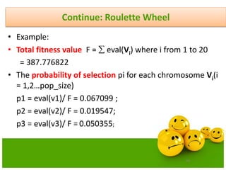
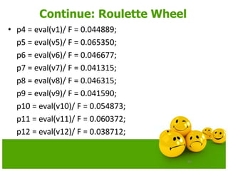
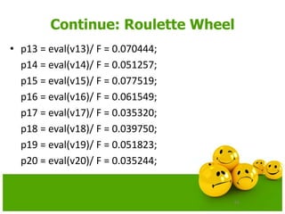
Continue: Roulette Wheel
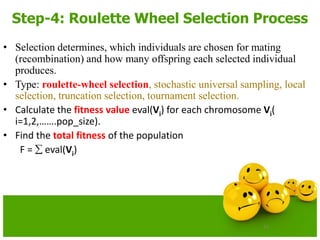
• Calculate the probability of a selection pi for each chromosome Vi
(I,2,……pop_size).
pi = eval(Vi)/ F
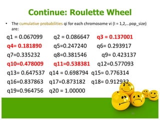
• Calculate the cumulative probability qi
for each chromosome Vi(I = 1,2,… pop_size);
qi =  pj where j varies from 1 to i
• Generate a random (float) number r from the range [0..1]
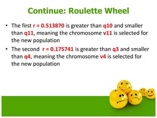
• If r<q1then select the first chromosome(v1); otherwise select the ith
chromosome Vi (2 i pop_size) such that q i-1 < r  qi.

59. 59
Continue: Roulette Wheel
• Example:
• Total fitness value F =  eval(Vi) where i from 1 to 20
= 387.776822
• The probability of selection pi for each chromosome Vi(i
= 1,2…pop_size)
p1 = eval(v1)/ F = 0.067099 ;
p2 = eval(v2)/ F = 0.019547;
p3 = eval(v3)/ F = 0.050355;

60. 60
Continue: Roulette Wheel
• p4 = eval(v1)/ F = 0.044889;
p5 = eval(v5)/ F = 0.065350;
p6 = eval(v6)/ F = 0.046677;
p7 = eval(v7)/ F = 0.041315;
p8 = eval(v8)/ F = 0.046315;
p9 = eval(v9)/ F = 0.041590;
p10 = eval(v10)/ F = 0.054873;
p11 = eval(v11)/ F = 0.060372;
p12 = eval(v12)/ F = 0.038712;

61. 61
Continue: Roulette Wheel
• p13 = eval(v13)/ F = 0.070444;
p14 = eval(v14)/ F = 0.051257;
p15 = eval(v15)/ F = 0.077519;
p16 = eval(v16)/ F = 0.061549;
p17 = eval(v17)/ F = 0.035320;
p18 = eval(v18)/ F = 0.039750;
p19 = eval(v19)/ F = 0.051823;
p20 = eval(v20)/ F = 0.035244;

62. 62
Continue: Roulette Wheel
• The cumulative probabilities qi for each chromosome vi (I = 1,2,…pop_size)
are:
q1 = 0.067099 q2 = 0.086647 q3 = 0.137001
q4= 0.181890 q5=0.247240 q6= 0.293917
q7=0.335232 q8=0.381546 q9= 0.423137
q10=0.478009 q11=0.538381 q12=0.577093
q13= 0.647537 q14 = 0.698794 q15= 0.776314
q16=0.837863 q17=0.873182 q18= 0.912932
q19=0.964756 q20 = 1.00000

63. 63
Continue: Roulette Wheel
• Let us assume that a (random) sequence of 20 numbers from the
range[0..1]is:
0.513870 0.175741 0.308652 0.534534 0.947628
0.171736 0.702231 0.226431 0.494773 0.424720
0.703899 0.389647 0.277226 0.368071 0.983437
0.005398 0.765682 0.646473 0.767139 0.780237

64. 64
Continue: Roulette Wheel
• The first r = 0.513870 is greater than q10 and smaller
than q11, meaning the chromosome v11 is selected for
the new population
• The second r = 0.175741 is greater than q3 and smaller
than q4, meaning the chromosome v4 is selected for
the new population

65. 65
Continue: Roulette Wheel
V1n=(011001111110110101100001101111000)(v11);
V2n=(100011000101101001111000001110010)(v4);
V3n=(001000100000110101111011011111011)(v7);
V4n=(011001111110110101100001101111000)(v11);
V5n=(000101010011111111110000110001100)(v19);
V6n=(100011000101101001111000001110010)(v4);
V7n=(111011101101110000100011111011110)(v15);
V8n=(000111011001010011010111111000101)(v5);
V9n=(011001111110110101100001101111000)(v11);
V10n=(000010000011001000001010111011101)(v3);

66. 66
Continue: Roulette Wheel
V11n=(111011101101110000100011111011110)(v15);
V12n=(010000000101100010110000001111100)(v9);
V13n=(000101000010010101001010111111011)(v6);
V14n=(100001100001110100010110101100111)(v8);
V15n=(101110010110011110011000101111110)(v20);
V16n=(100110100000001111111010011011111)(v1);
V17n=(000001111000110000011010000111011)(v10);
V18n=(111011111010001000110000001000110)(v13);
V19n=(111011101101110000100011111011110)(v15);
V20n=(110011110000011111100001101001011)(v16);

67. Step-5:Recombination(Crossover )
6/21/2013 67
Recombination produces new individuals in combining
the information contained in the parents (parents - mating
population).
 Type: Discrete recombination
Real valued recombination,
Binary valued recombination,
single-point / double-point /multi-point crossover,
uniform crossover,
shuffle crossover,
crossover with reduced surrogate,

68. 68
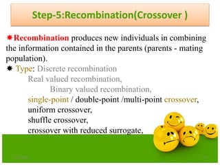
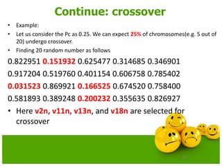
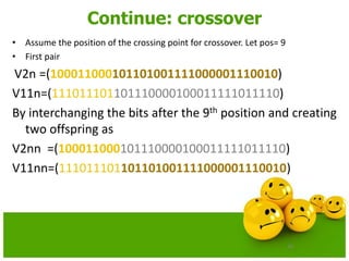
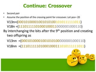
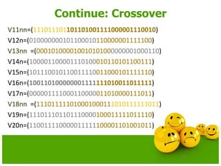
Continue: Crossover
• Assume the probability of crossover Pc.
• This probability gives us the expected number Pc*
pop_size of chromosomes which undergo the
crossover operation.
• Generate a random(float) number r from the
range[0..1]
• If r<Pc, select the given chromosome for
crossover

69. 69
Continue: crossover
• Example:
• Let us consider the Pc as 0.25. We can expect 25% of chromosomes(e.g. 5 out of
20) undergo crossover.
• Finding 20 random number as follows
0.822951 0.151932 0.625477 0.314685 0.346901
0.917204 0.519760 0.401154 0.606758 0.785402
0.031523 0.869921 0.166525 0.674520 0.758400
0.581893 0.389248 0.200232 0.355635 0.826927
• Here v2n, v11n, v13n, and v18n are selected for
crossover

70. 70
Continue: crossover
• Assume the position of the crossing point for crossover. Let pos= 9
• First pair
V2n =(100011000101101001111000001110010)
V11n=(111011101101110000100011111011110)
By interchanging the bits after the 9th position and creating
two offspring as
V2nn =(100011000101110000100011111011110)
V11nn=(111011101101101001111000001110010)

71. 71
Continue: Crossover
• Second pair
• Assume the position of the crossing point for crossover. Let pos= 20
V13n=(000101000010010101001010111111011)
V18n =(111011111010001000110000001000110)
By interchanging the bits after the 9th position and creating
two offspring as
V13nn =(000101000010010101000000001000110)
V18nn =(111011111010001000111010111111011)

72. 72
Continue: Crossover
V1n=(011001111110110101100001101111000)
V2nn =(100011000101110000100011111011110)
V3n=(001000100000110101111011011111011)
V4n=(011001111110110101100001101111000)
V5n=(000101010011111111110000110001100)
V6n=(100011000101101001111000001110010)
V7n=(111011101101110000100011111011110)
V8n=(000111011001010011010111111000101)
V9n=(011001111110110101100001101111000)
V10n=(000010000011001000001010111011101)

73. 73
Continue: Crossover
V11nn=(111011101101101001111000001110010)
V12n=(010000000101100010110000001111100)
V13nn =(000101000010010101000000001000110)
V14n=(100001100001110100010110101100111)
V15n=(101110010110011110011000101111110)
V16n=(100110100000001111111010011011111)
V17n=(000001111000110000011010000111011)
V18nn =(111011111010001000111010111111011)
V19n=(111011101101110000100011111011110)
V20n=(110011110000011111100001101001011)

74. Step-6: Mutation
6/21/2013 74
 After recombination every offspring undergoes mutation.
Offspring variables are mutated by small perturbations (size of the
mutation step), with low probability. The representation of the
variables determines the used algorithm.
Type:
Mutation operator for real valued variables
Mutation for binary valued variables

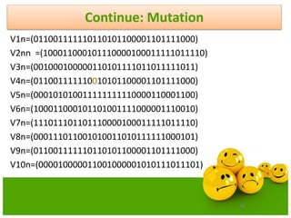
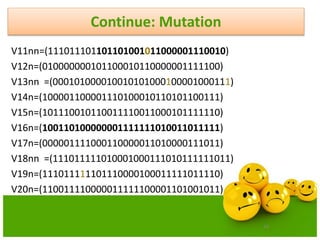
75. 75
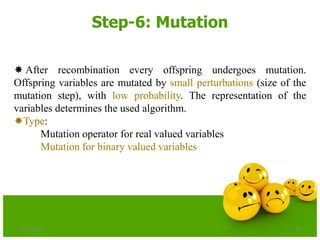
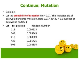
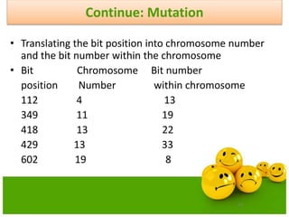
Continue: Mutation
• Mutation is performed bit-by-bit basis
• Assume the probability of Mutation Pm.
• This probability gives us the expected number of
mutated bits Pm* pop_size.
• Generate a random(float) number r from the
range[0..1]
• If r<Pm, mutate the bit

76. 76
Continue: Mutation
• Example:
• Let the probability of Mutation Pm = 0.01. This indicates 1% of
bits would undergo Mutation. Here 0.01* 33*20 = 6.6 number of
bits will be mutated
• Let Bit position Random Number
112 0.000213
349 0.009945
418 0.008809
429 0.005425
602 0.002836

77. 77
Continue: Mutation
• Translating the bit position into chromosome number
and the bit number within the chromosome
• Bit Chromosome Bit number
position Number within chromosome
112 4 13
349 11 19
418 13 22
429 13 33
602 19 8

78. 78
Continue: Mutation
V1n=(011001111110110101100001101111000)
V2nn =(100011000101110000100011111011110)
V3n=(001000100000110101111011011111011)
V4n=(011001111110010101100001101111000)
V5n=(000101010011111111110000110001100)
V6n=(100011000101101001111000001110010)
V7n=(111011101101110000100011111011110)
V8n=(000111011001010011010111111000101)
V9n=(011001111110110101100001101111000)
V10n=(000010000011001000001010111011101)

79. 79
Continue: Mutation
V11nn=(111011101101101001011000001110010)
V12n=(010000000101100010110000001111100)
V13nn =(000101000010010101000100001000111)
V14n=(100001100001110100010110101100111)
V15n=(101110010110011110011000101111110)
V16n=(100110100000001111111010011011111)
V17n=(000001111000110000011010000111011)
V18nn =(111011111010001000111010111111011)
V19n=(111011111101110000100011111011110)
V20n=(110011110000011111100001101001011)

80. 80
Step-7: Evaluation of Result
• Decode each chromosome and calculate the fitness function values from <x1,
x2> values just decoded
• Eval(v1) = f(3.130078, 4.996097) = 23.410669;
Eval(v2) = f(5.279042, 5.054515) = 18.201083;
Eval(v3) = f(-0.991471, 5.680258) = 16.020812 ;
Eval(v4) = f(3.128235, 4.996097) = 23.412613;
Eval(v5) = f( -1.746635, 5.395584) = 20.095903;

81. 81
continue: Evaluation of Result
Eval(v6) = f( 5.278638,5.593460) =17.406725 ;
Eval(v7) = f( 11.089025, 5.054515) = 30.060205 ;
Eval(v8) = f(-1.255173, 4.734458) = 25.341160;
Eval(v9) = f(3.130078, 4.996097) = 23.410669 ;
Eval(v10) = f( -2.516603, 4.390381) =19.526329 ;
Eval(v11) = f(11.088621, 4.743434) = 33.351874 ;
Eval(v12) = f(0.795406, 5.381472) = 16.127799 ;
Eval(v13) = f(-1.811725, 4.209937) = 22.692462 ;
Eval(v14) = f(4.910618, 4.703018) = 17.959701 ;

82. 82
continue: Evaluation of Result
• Eval(v15) = f(7.935998, 4.757338) = 13.666916;
Eval(v16) = f(6.084492, 5.652242) = 26.019600 ;
Eval(v17) = f(-2.554851, 4.793707) = 21.278435;
Eval(v18) = f(11.134646, 5.666976) = 27.591064 ;
Eval(v19) = f( 11.059532, 5.054515) = 27.608441 ;
Eval(v20) = f(9.211598, 4.993762) = 23.867227 ;

83. 83
continue: Evaluation of Result
• The total fitness of the new population is f = 447.049688,
much higher than the total fitness of the previous
population 387.776822
• The best chromosome now v11 has a better evaluation
33.351874 than the best chromosome v15 from the
previous population(30.060205)

84. 84
PSO and GA Comparison
• Commonalities
– PSO and GA are both population based stochastic optimization
– both algorithms start with a group of a randomly generated
population,
– both have fitness values to evaluate the population.
– Both update the population and search for the optimium with
random techniques.
– Both systems do not guarantee success.
6/21/2013

85. 85
PSO and GA Comparison
• Differences
– PSO does not have genetic operators like crossover and
mutation. Particles update themselves with the internal
velocity.
– They also have memory, which is important to the algorithm.
– Particles do not die
– the information sharing mechanism in PSO is significantly
different
• Info from best to others, GA population moves together
6/21/2013

86. 86
• PSO has a memory
not “what” that best solution was, but “where” that best solution
was
• Quality: population responds to quality factors pbest and gbest
• Diverse response: responses allocated between pbest and gbest
• Stability: population changes state only when gbest changes
• Adaptability: population does change state when gbest changes
6/21/2013

87. 87
• There is no selection in PSO
all particles survive for the length of the run
PSO is the only EA that does not remove candidate population
members
• In PSO, topology is constant; a neighbor is a neighbor
• Population size: 20-40
6/21/2013

88. Multi-objective Optimization: Concepts
and Application to Data mining

89. Multi-objective Optimization
• “Multiobjective optimization is the process of simultaneously
optimizing two or more conflicting objectives subject to
certain constraints.”
Examples:
– Maximizing profit and minimizing the cost of a product.
– Maximizing performance and minimizing fuel consumption of
a vehicle.
– Minimizing weight while maximizing the strength of a
particular component

90. 6/21/2013 90
]10,0[
2010
;)10()(
;)(
2
2
2
1




x
utionOptimalSol
x
where
xxf
xxf
Minimize

91. Standard Approach: Weighted Sum of Objective
6/21/2013 91

92. Difference
Single Objective Optimization
– Optimize only one objective function
– Single optimal solution
– Maximum/Minimum fitness value is selected as the best
solution.
Multiobjective Optimization
– Optimize two or more than two objective functions
– Set of optimal solutions
– Comparison of solutions by
• Domination
• Non-domination

93. Pareto Optimal Solutions
6/21/2013 93
Max-max
Max-min
Function-1
Function-2 Min-max
Min- Min

94. Flowchart of NSGA-II

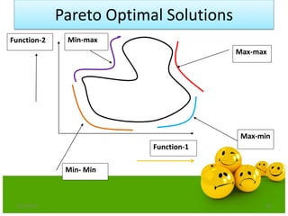
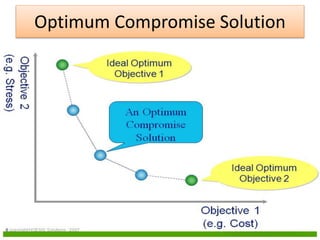
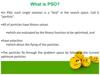
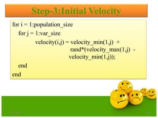
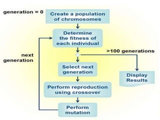
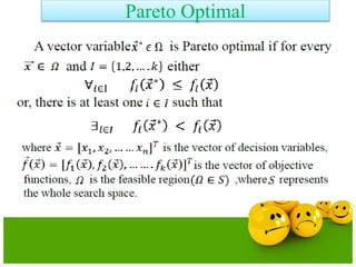
95. Definitions
Domination: One solution is said to
dominate another if it is better in all
objectives.
Non-Domination[Pareto points]: A solution
is said to be non-dominated if it is better
than other solutions in at least one
objective
•A dominates B (better in both ƒ1 and ƒ2)
•A dominates C (same in ƒ2 but better in ƒ1)
•A does not dominate D (non-dominated points)
•A and D are in the “Pareto optimal front”
•These non-dominated solutions are called Pareto optimal solutions.
•This non-dominated curve is said to be Pareto front.

96. Desirable MOEA features
• Convergence: Convergence refers to how close is the
approximation to the Optimal Pareto Front.
• Diversity: Diversity refers to how well distributed are the elements
of the approximation among the Pareto Front
A multi-objective optimization
algorithm must achieve:
1. Guide the search towards the
global Pareto-Optimal front.(By
non-domination ranking )
2. Maintain solution diversity in
the Pareto-Optimal front. ( by
Crowding Distance)

97. Non Dominated Sorting based Genetic
Algorithm II (NSGA-II)
• Famous for Fast non-dominated search.
• Fitness assignment-Ranking based on non-domination sorting.
• Diversity mechanism is based on Crowding distance.
• Uses Elitism (A practical variant of the general process of
constructing a new population is to allow the best organism(s)
from the current generation to carry over to the next, unaltered.
This strategy is known as elitist selection and guarantees that the
solution quality obtained by the GA will not decrease from one
generation to the next)

98. Initialize Population
6/21/2013 98
Maximize
F1(x1,x2)=21.5+x1*sin(4*π*x1)+x2*sin(20*π*x
2)
F2(x1,x2)=21.5+x1*cos(4*π*x1)+x2*cos(20*π*
x2)
Where
-3<=x1<=12.1
4.1<=x2<=5.8
 Let us choose 10 random value for x1 and x2.
Initialize population with10 chromosomes having
single dimensioned real value.
x1 x2
0.8968 4.7948
5.9829 4.5458
6.1029 5.3091
0.3484 4.2996
1.4798 4.6419
3.4049 4.9643
-1.7087 4.5462
9.0953 4.1497
11.0257 5.3416
4.3780 5.0835

99. Evaluate Fitness values
F1(x1,x2) F2(x1,x2)
19.1045 26.2858
21.4232 22.9604
30.2333 27.6415
21.0656 25.6839
23.3844 18.8755
14.6390 19.4350
23.4170 18.5652
30.0549 20.6653
27.6999 27.3475
12.7483 24.2504
After calculating F1 and F2 for each solution we will get the
following fitness values

100. Pareto Optimal
  ii uvni  :,,1 

101. 6/21/2013 101
F1 F2 Index Dominated By Rank
19.1045 26.2858 1 3,9 3
21.4232 22.9604 2 3,9 3
30.2333 27.6415 3 NIL 1
21.0656 25.6839 4 3,9 3
23.3844 18.8755 5 3,8,9 4
14.6390 19.4350 6 1,2,3,4,8,9 6
23.4170 18.5652 7 3,8,9 4
30.0549 20.6653 8 3 2
27.6999 27.3475 9 3 2
12.7483 24.2504 10 1,3,4,9 5
Ranking

102. Fast Non-domination Sorting

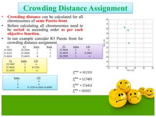
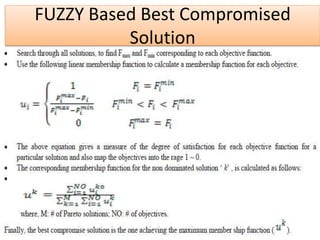
103. Crowding Distance Assignment
• To get an estimate of density of
solutions surrounding a particular
solution in population.
• Choose individuals having large
crowding distance.
• Help for obtaining uniformly
distribution
where ƒ[i]m represent objective function value of solution. and are
the maximum and minimum value of the objective function.

104. Crowding Distance Assignment
• Crowding distance can be calculated for all
chromosomes of same Pareto front.
• Before calculating all chromosomes need to
be sorted in ascending order as per each
objective function.
• In our example consider R3 Pareto front for
crowding distance assignment
F1 F2 Index Rank
19.1045 26.2858 1 3
21.4232 22.9604 2 3
21.0656 25.6839 4 3
F1 Index CD
19.1045 1 ∞
21.0656 4 0.1326
21.4232 2 ∞
F2 Index CD
22.9604 2 ∞
25.6839 4 0.3663
26.2858 1 ∞
Index CD
1 ∞
2 ∞
4 0.1326+0.3663=0.4989

105. Tournament Selection
Selection is the stage of a genetic algorithm in which individual are
chosen from a population for later breeding(recombination or
crossover).
Crowded-Comparison Operator:
• The crowded-comparison operator guides the selection process
at the various stages of the algorithm toward a uniformly spread-out
Pareto optimal front.
n

106. 6/21/2013 106
Based on Crowding Distance

107. New Generation Formation
• After sorting as per non-domination all solutions will go
through binary selection, Recombination and mutation to
generate Qt.
• Unite old population Pt and present population Qt (Elitism is
preserved). Now we have 2N number of solutions.
• So these 2N solutions are again to be sorted as per non-
domination to bring the better solutions to higher front.

108. Contd…
• Now we have to select top N number of solutions as per non-
domination and crowding distance.
• Add each front (according to the rank or pareto front ) to new
population Pt+1 until |Pt+1| ≤ N.
• If |Pt+1|=N then no more solutions from next front can be added.
• If |Pt+1|<N few more solutions need to be added to Pt+1. Now
which solutions from next front is to be added that can be decided
by crowding distance as all solutions of that front are of same
rank/level.

109. Parent
Child
Parent
Child
Combined
PopulationNon-dominated
sorting
Crowding distance
sorting
F1
F2
F3
Parent
Child
Combined
Population
Overview of NSGA II

110. Optimum Compromise Solution
6/21/2013 110

111. FUZZY Based Best Compromised
Solution
6/21/2013 111

112. Application of Multi-objective for Data Mining
6/21/2013 112
Multi-objective Data Mining
Feature Selection
Classification
Clustering
Association Rule Mining

113. 6/21/2013 113