LEAST MEAN SQUARE
AND
GEOMETRIC TRANFORMATION
PRESENTED BY,
K.LALITHAMBIGA,
II- M.Sc (CS & IT),
Nadar Saraswathi College of
Arts and Science, Theni.
SYNOPSIS
 Minimum Mean Square Error Filtering
or
 Least Square Error Filtering
 Constrained Least Square Filtering
 Geometric Transformation
 Spatial Transformation
 Geometric Distortion
 Gray Level Interpolation
 Nearest Neighbor Gray Level Interpolation
 Bilinear Interpolation
MINIMUM MEAN SQUARE ERROR (WIENER)
FILTERING
 In most images, adjacent pixels are highly correlated, while the
gray level of widely separated pixels are only loosely correlated.
 Therefore, the autocorrelation function of typical images
generally decreases away from the origin.
 Power spectrum of an image is the Fourier transform of its
autocorrelation function, therefore we can argue that the power
spectrum of an image generally decreases with frequency.
 Typical noise sources have either a flat power spectrum or one
that decreases with frequency more slowly than typical image
power spectrum.
 Therefore, the expected situation is for the signal to dominate the
spectrum at low frequencies, while the noise dominates the high
frequencies.
MINIMUM MEAN SQUARE ERROR (WIENER)
FILTERING
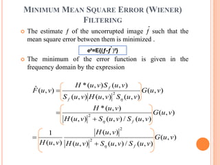
 The estimate ƒ of the uncorrupted image ƒ such that the
mean square error between them is minimized .
 The minimum of the error function is given in the
frequency domain by the expression
e²=E{(ƒ-ƒ )²}ˆ
),(
),(/),(),(
),(
),(
1
),(
),(/),(),(
),(*
),(
),(),(),(
),(),(*
),(ˆ
2
2
2
2
vuG
vuSvuSvuH
vuH
vuH
vuG
vuSvuSvuH
vuH
vuG
vuSvuHvuS
vuSvuH
vuF
f
f
f
f








ˆ
MINIMUM MEAN SQUARE ERROR
(WIENER) FILTERING
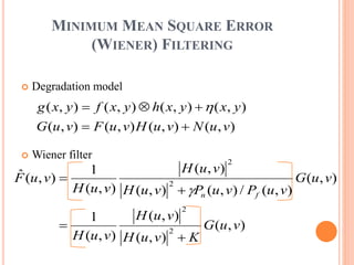
 Degradation model
 Wiener filter
),(),(),(),(
),(),(),(),(
vuNvuHvuFvuG
yxyxhyxfyxg

 
),(
),(
),(
),(
1
),(
),(/),(),(
),(
),(
1
),(ˆ
2
2
2
2
vuG
KvuH
vuH
vuH
vuG
vuPvuPvuH
vuH
vuH
vuF
fn





MINIMUM MEAN SQUARE ERROR
(WIENER) FILTERING
MINIMUM MEAN SQUARE ERROR (WIENER)
FILTERING
WIENER FILTERING - PROBLEMS
 The power spectra of the under graded image and noise
must be known.
 Weights all errors equally regardless of their location in the
image, while the eye is considerably more tolerant of errors
in the dark areas and high-gradient areas in the image.
 In minimizing the mean square error, Wiener filter also
smooth the image more than the eye would prefer
CONSTRAINED LEAST SQUARES
FILTERING
Only the mean and variance of the noise is required
g-vector by using the image elements in first row of g(x,y)
-dimensions
H –The matrix H then has dimensions MNX MN
The degradation model in vector-matrix form
The objective function
Subject to the constraint
111   MNMNMNMNMN ηfHg
21
0
1
0
2
)],([





M
x
N
y
yxfC
ηHfg 
ηf,
22
ηHfg 
CONSTRAINED LEAST SQUARES
FILTERING
The frequency domain solution to this optimization
problem
The Fourier transform of the function
),(
),(),(
),(*
),(ˆ
2
vuG
vuPvuH
vuH
vuF
















010
141
010
),( yxp
CONSTRAINED LEAST SQUARES
FILTERING - EXAMPLE
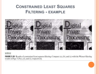
Low noise: Wiener and CLS generate
equal results.
High noise: CLS outperforms Wiener if λ
is properly selected.
It is easier to select the scalar value for λ
than to approximate the SNR which is
seldom constant
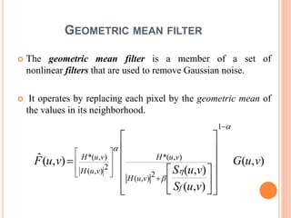
GEOMETRIC MEAN FILTER
 The geometric mean filter is a member of a set of
nonlinear filters that are used to remove Gaussian noise.
 It operates by replacing each pixel by the geometric mean of
the values in its neighborhood.
),(
),(
),(
),(ˆ
2
),(
),(*
1
2),(
),(*
vuG
vuS
vuS
vuF
f
vuH
vuH
vuH
vuH

































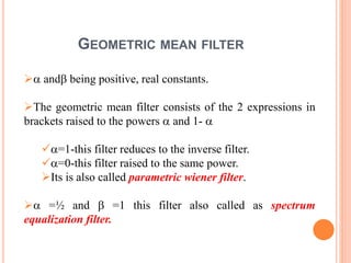
GEOMETRIC MEAN FILTER
 and being positive, real constants.
The geometric mean filter consists of the 2 expressions in
brackets raised to the powers  and 1- 
=1-this filter reduces to the inverse filter.
=0-this filter raised to the same power.
Its is also called parametric wiener filter.
 =½ and  =1 this filter also called as spectrum
equalization filter.
GEOMETRIC TRANSFORMATIONS
 The geometric transformations modify the spatial
relationships between pixels in an image.
 The geometric transformations often are called rubber-
sheet transformations
 Geometric transformation consists of 2 basic operations:
1. A Spatial Transformations –rearrangement of pixels on
the image plane.
2. Gray-level interpolation –assignment of gray levels to
pixels in the spatially transformed image.
SPATIAL TRANSFORMATION
 Assume the original image f(x,y) is subject to geometric
distortion yielding g(x’,y’)
 Spatial transformation &
 Coordination transformation
 The most frequently to overcome this difficulty is to formulate
the spatial relocation of pixels by the use of tiepoints,
 Subset of pixels whose location
 Input – Distorted
 Output – Corrected
• Function need 8 or more points
to find {ci; 1  i  8}
x´=r(x,y) y´=s(x,y)
8765
4321
),('
),('
cxycycxcyxsy
cxycycxcyxrx


GRAY LEVEL INTERPOLATION
 Spatial transformations establish a correspondence between
a point (x’, y’) in the distorted image g(x’,y’) and original
image f(x,y).
 To correct the geometric transformation, one needs to
estimate gray values of f(x,y),
 If x’ and y’ are integers, then
 If x’ and y’ are fraction numbers, but fall within the b order
of the original image, then interpolation will be needed to
find
 The gray-level interpolation is based on a nearest neighbor
approach. The method is called zero order interpolation.
),(ˆ yxf
)','(),(ˆ yxgyxf 
),(ˆ yxf
NEAREST NEIGHBOR GRAY LEVEL
INTERPOLATION
   )','(),(ˆ yxgyxf 
BILINEAR INTERPOLATION
 Estimate the value of =g(x’,y’)) using
four nearest neighbors when x’ and y’ are
fractional numbers.
 Substitute g(x1,y1), g(x1,y2), g(x2,y1), g(x2,y2)
into above equation and solve for a, b, c, d.
It’s 4 equations and 4 unknowns.
(x1,y2)
(x1,y1)
(x2,y2)
(x2,y1)
   
   
dycxbyaxyxg
yyyyy
xxxxx



'''')','(and
'''
'''
21
21
(x’,y’)
),(ˆ yxf
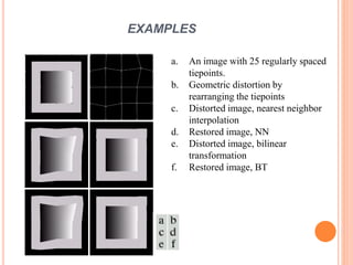
a. An image with 25 regularly spaced
tiepoints.
b. Geometric distortion by
rearranging the tiepoints
c. Distorted image, nearest neighbor
interpolation
d. Restored image, NN
e. Distorted image, bilinear
transformation
f. Restored image, BT
EXAMPLES
EXAMPLES
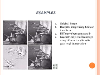
a. Original image
b. Distorted image using bilinear
transform
c. Difference between a and b
d. Geometrically restored image
using bilinear transform for
gray level interpolation
Digital Image Processing

Digital Image Processing

  • 1.
    LEAST MEAN SQUARE AND GEOMETRICTRANFORMATION PRESENTED BY, K.LALITHAMBIGA, II- M.Sc (CS & IT), Nadar Saraswathi College of Arts and Science, Theni.
  • 2.
    SYNOPSIS  Minimum MeanSquare Error Filtering or  Least Square Error Filtering  Constrained Least Square Filtering  Geometric Transformation  Spatial Transformation  Geometric Distortion  Gray Level Interpolation  Nearest Neighbor Gray Level Interpolation  Bilinear Interpolation
  • 3.
    MINIMUM MEAN SQUAREERROR (WIENER) FILTERING  In most images, adjacent pixels are highly correlated, while the gray level of widely separated pixels are only loosely correlated.  Therefore, the autocorrelation function of typical images generally decreases away from the origin.  Power spectrum of an image is the Fourier transform of its autocorrelation function, therefore we can argue that the power spectrum of an image generally decreases with frequency.  Typical noise sources have either a flat power spectrum or one that decreases with frequency more slowly than typical image power spectrum.  Therefore, the expected situation is for the signal to dominate the spectrum at low frequencies, while the noise dominates the high frequencies.
  • 4.
    MINIMUM MEAN SQUAREERROR (WIENER) FILTERING  The estimate ƒ of the uncorrupted image ƒ such that the mean square error between them is minimized .  The minimum of the error function is given in the frequency domain by the expression e²=E{(ƒ-ƒ )²}ˆ ),( ),(/),(),( ),( ),( 1 ),( ),(/),(),( ),(* ),( ),(),(),( ),(),(* ),(ˆ 2 2 2 2 vuG vuSvuSvuH vuH vuH vuG vuSvuSvuH vuH vuG vuSvuHvuS vuSvuH vuF f f f f         ˆ
  • 5.
    MINIMUM MEAN SQUAREERROR (WIENER) FILTERING  Degradation model  Wiener filter ),(),(),(),( ),(),(),(),( vuNvuHvuFvuG yxyxhyxfyxg    ),( ),( ),( ),( 1 ),( ),(/),(),( ),( ),( 1 ),(ˆ 2 2 2 2 vuG KvuH vuH vuH vuG vuPvuPvuH vuH vuH vuF fn     
  • 6.
    MINIMUM MEAN SQUAREERROR (WIENER) FILTERING
  • 7.
    MINIMUM MEAN SQUAREERROR (WIENER) FILTERING
  • 8.
    WIENER FILTERING -PROBLEMS  The power spectra of the under graded image and noise must be known.  Weights all errors equally regardless of their location in the image, while the eye is considerably more tolerant of errors in the dark areas and high-gradient areas in the image.  In minimizing the mean square error, Wiener filter also smooth the image more than the eye would prefer
  • 9.
    CONSTRAINED LEAST SQUARES FILTERING Onlythe mean and variance of the noise is required g-vector by using the image elements in first row of g(x,y) -dimensions H –The matrix H then has dimensions MNX MN The degradation model in vector-matrix form The objective function Subject to the constraint 111   MNMNMNMNMN ηfHg 21 0 1 0 2 )],([      M x N y yxfC ηHfg  ηf, 22 ηHfg 
  • 10.
    CONSTRAINED LEAST SQUARES FILTERING Thefrequency domain solution to this optimization problem The Fourier transform of the function ),( ),(),( ),(* ),(ˆ 2 vuG vuPvuH vuH vuF                 010 141 010 ),( yxp
  • 11.
  • 12.
    Low noise: Wienerand CLS generate equal results. High noise: CLS outperforms Wiener if λ is properly selected. It is easier to select the scalar value for λ than to approximate the SNR which is seldom constant
  • 13.
    GEOMETRIC MEAN FILTER The geometric mean filter is a member of a set of nonlinear filters that are used to remove Gaussian noise.  It operates by replacing each pixel by the geometric mean of the values in its neighborhood. ),( ),( ),( ),(ˆ 2 ),( ),(* 1 2),( ),(* vuG vuS vuS vuF f vuH vuH vuH vuH                                 
  • 14.
    GEOMETRIC MEAN FILTER and being positive, real constants. The geometric mean filter consists of the 2 expressions in brackets raised to the powers  and 1-  =1-this filter reduces to the inverse filter. =0-this filter raised to the same power. Its is also called parametric wiener filter.  =½ and  =1 this filter also called as spectrum equalization filter.
  • 15.
    GEOMETRIC TRANSFORMATIONS  Thegeometric transformations modify the spatial relationships between pixels in an image.  The geometric transformations often are called rubber- sheet transformations  Geometric transformation consists of 2 basic operations: 1. A Spatial Transformations –rearrangement of pixels on the image plane. 2. Gray-level interpolation –assignment of gray levels to pixels in the spatially transformed image.
  • 16.
    SPATIAL TRANSFORMATION  Assumethe original image f(x,y) is subject to geometric distortion yielding g(x’,y’)  Spatial transformation &  Coordination transformation  The most frequently to overcome this difficulty is to formulate the spatial relocation of pixels by the use of tiepoints,  Subset of pixels whose location  Input – Distorted  Output – Corrected • Function need 8 or more points to find {ci; 1  i  8} x´=r(x,y) y´=s(x,y) 8765 4321 ),(' ),(' cxycycxcyxsy cxycycxcyxrx  
  • 17.
    GRAY LEVEL INTERPOLATION Spatial transformations establish a correspondence between a point (x’, y’) in the distorted image g(x’,y’) and original image f(x,y).  To correct the geometric transformation, one needs to estimate gray values of f(x,y),  If x’ and y’ are integers, then  If x’ and y’ are fraction numbers, but fall within the b order of the original image, then interpolation will be needed to find  The gray-level interpolation is based on a nearest neighbor approach. The method is called zero order interpolation. ),(ˆ yxf )','(),(ˆ yxgyxf  ),(ˆ yxf
  • 18.
    NEAREST NEIGHBOR GRAYLEVEL INTERPOLATION    )','(),(ˆ yxgyxf 
  • 19.
    BILINEAR INTERPOLATION  Estimatethe value of =g(x’,y’)) using four nearest neighbors when x’ and y’ are fractional numbers.  Substitute g(x1,y1), g(x1,y2), g(x2,y1), g(x2,y2) into above equation and solve for a, b, c, d. It’s 4 equations and 4 unknowns. (x1,y2) (x1,y1) (x2,y2) (x2,y1)         dycxbyaxyxg yyyyy xxxxx    '''')','(and ''' ''' 21 21 (x’,y’) ),(ˆ yxf
  • 20.
    a. An imagewith 25 regularly spaced tiepoints. b. Geometric distortion by rearranging the tiepoints c. Distorted image, nearest neighbor interpolation d. Restored image, NN e. Distorted image, bilinear transformation f. Restored image, BT EXAMPLES
  • 21.
    EXAMPLES a. Original image b.Distorted image using bilinear transform c. Difference between a and b d. Geometrically restored image using bilinear transform for gray level interpolation