This document provides an overview of digital image processing. It discusses key topics including digital image fundamentals, image transforms, image enhancement, image restoration, image compression, image segmentation, representation and description, and recognition and interpretation. The document outlines concepts and techniques within each of these topics at a high level over multiple sections and pages with headings, content lists, and explanatory diagrams.

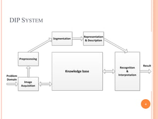
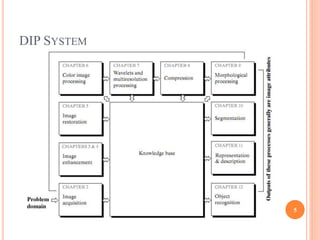
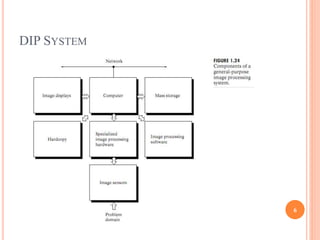
1. DIGITAL IMAGE PROCESSING
PART I
Thuong Nguyen1

2. CONTENT
 Digital image fundamentals
 Image transform
 Image enhancement
 Image restoration
 Image compression
2

3. I. DIGITAL FUNDAMENTAL
 Digital Image Processing System
 Sampling and Quantization
 Relationships between pixels
3

4. DIP SYSTEM
4

5. DIP SYSTEM
5

6. DIP SYSTEM
6

7. SAMPLING AND QUANTIZATION
 Quantization: limit of intensity resolution
 Sampling: Limit of spatial and temp resolution
 Uniform and non-uniform
7

8. PIXEL’S RELATIONSHIPS
 Two pixel are adjacent if
 Neighbors as 4, 8, and m-connectivity
 Gray levels satisfy a specified criterion
 Connectivity
 Existing a path between two pixels
 Path
 Path from p(x,y) to q(s,t) is
Where (x, y) = (x0, y0), (s, t) = (xn, yn)
8
(x0, y0), (x1, x2), …, (xn, yn)

9. II. IMAGE ENHANCEMENT IN FREQ DOMAIN
 Discrete Fourier Transform
 Other Image Transform
 Hotelling Transform
9

10. THE DISCRETE FOURIER TRANSFORM
 The Fourier transform
 1-D
 2-D
 Properties
10

11. THE DISCRETE FOURIER TRANSFORM
 Discrete Fourier transform pair
 One dimensional
 Two dimensional
11

12. THE DISCRETE FOURIER TRANSFORM
 2D FFT and Image Processing
12

13. THE DISCRETE FOURIER TRANSFORM
1. Multiply input image by −1 𝑥+𝑦
2. Compute 𝐹(𝑢, 𝑣), DFT
3. Multiply 𝐹(𝑢, 𝑣) by 𝐻 𝑢, 𝑣
4. Compute IDFT
5. Obtain the real part
6. Multiply the result by −1 𝑥+𝑦
13
 Fast Fourier transform
 Efficient algorithm to compute DFT by reduce computation
burden: O(N2) – O(NlogN)

14. OTHER SEPARABLE IMAGE TRANSFORM
 General relation ship
 Several condition
 Separable
 Symmetric
 Separable kernel can be compute in two step of 1D transf
 For separable and symmetric kernel
14

15. OTHER SEPARABLE IMAGE TRANSFORM
 Walsh Transform
 Hadamard transform
 Discrete cosine transform
15

16. HOLTELLING TRANSFORM
16
1
2
.
.
n
x
x
x
x
 
 
 
 
 
 
  
1
1
{ }
M
x k
k
m E x x
M 
  
x,........,
M data points
1 M
1
1
{( )( ) }
M
T TT
x x x k k k k
k
C E x m x m x x m m
M 
    
Mean:
Covariance:

17. III. IMAGINE ENHANCEMENT
 Basic intensity functions
 Histogram processing
 Spatial Filtering
 Enhancement in the Frequency domain
 Color image processing
17

18. BASIC INTENSITY FUNCTIONS
 Spatial domain process
 Image negatives:
 intensity level in the range [0, L-1]
 s = L – 1 – r
 Log trans
 s = c log(1 + r)
 Power law (gramma) trans
 s = c r
 Piecewise-Linear Trans
 Contrast stretching
 Intensity level slicing
 Bit plane slicing
18

19. HISTOGRAM PROCESSING
 Histogram
 Histogram equalization:
 Histogram matching
 Local histogram processing
 Image subtraction
 Image averaging
19

20. SPATIAL FILTERING
 Fundamental: using spatial masks for Image Processing
 Smoothing Filter
 Lowpass spatial filtering
 Meadian filtering
20

21. SPATIAL FILTERING
 Sharpening filter
 Highpass spatial filtering
 Emphasize fine details
 High-boost filtering
 Enhance high freq while keeping the low freq
 Highboost = (A-1) original + Highpass
 Derivative filters
 First order: gradient
 Second order
21

22. ENHANCEMENT IN THE FREQUENCY DOMAIN
Spatial domain
 Definition
 Chang pixel position  changes
in the scene
 Distance is real
 Processing
 Directly process the input image
pixel array
22
Frequency domain
 Definition
 Change in image position 
changes in spatial frequency
 Which image intensity values are
changing in the spatial domain
image
 Processing
 Transform the image to its
frequency representation
 Perform image processing
 compute

23. ENHANCEMENT IN THE FREQUENCY DOMAIN
 Lowpass filter
 Ideal
 Butterword
 Highpass filter
 Ideal
 Butterworth
 Homomorphic
23

24. COLOR IMAGE PROCESSING
 Background
 Human can perceive thousands of colors
 Two major area: full color and pseudo color
 Color quantization: 8-bit or 24bit
 Color fundamental
 Result of light in the rentina: 400-700nm
 Characterization of light: monochromatic and gray level
 Radiance: total amount of energy emitted by light source
 Brightness: intensity
 Luminance: amount of energy perceived by obervers, in lumens
 Color characters
 Hue
 Saturation
 Birghtness 24

25. IV. IMAGE RESTORATION
 Degradation Model
 Diagonalization of Circulant & Block-Circulant Matrices
 Algebraic Approach
 Inverse Filtering
 Weiner Filter
 Constrained LS Restoration
 Interactive Restoration
 Restoration at Spatial Domain
 Geometric transform
25

26.  Noise models
 Spatial and frequency properties
 Noise PDF: Gaussian, Rayleigh, Erlang, Exponential, Uniform,
Impulse ..
 Estimate noise parameters:
 Spectrum inspection: periodic noise
 Test image: mean, variance and histogram shape, if imaging system is
available
 De-noising
 Spatial filtering ( for additive noise)
 Mean filters
 Order-statistics filters
 Adaptive filters:
 Frequency domain filtering (for periodic noise)
DEGRADATION MODEL
26

27. V. IMAGE COMPRESSION
 Fundamentals
 Image Compression Models
 Elements of Information Theory
 Error-Free Compression
 Lossy Compression
 Image Compression standard
27

28. VI. IMAGE SEGMENTATION
 Detection of Discontiuties
 Edge Linking and Boundary Detection
 Thresholding
 Region-Oriented Segmentation
 Motion in Segmentation
28

29. VII. REPRESENTATION AND DESCRIPTION
 Representation Scheme
 Boundary Descriptors
 Regional Descriptors
 Morphology
 Relational Descriptors
29

30. VIII. RECOGNITION AND INTERPRETATION
 Elements of Image Analysis
 Patterns and Pattern Classes
 Decision-Theoretic Methods
 Structural Methods
 Interpretation
30