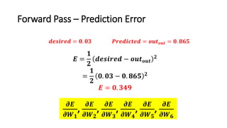
Downloaded 985 times


![Weights Update Equation
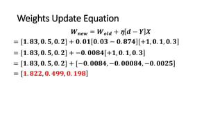
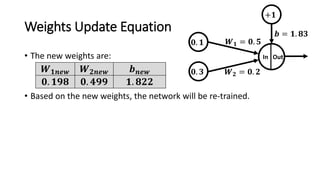
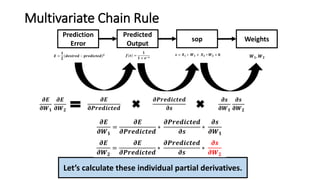
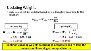
• We can use the weights update equation:
𝑾 𝒏𝒆𝒘: new updated weights.
𝑾 𝒐𝒍𝒅: current weights. [1.83, 0.5, 0.2]
η: network learning rate. 0.01
𝒅: desired output. 0.03
𝒀: predicted output. 0.874
𝑿: current input at which the network made false prediction. [+1, 0.1, 0.3]
𝑾 𝒏𝒆𝒘 = 𝑾 𝒐𝒍𝒅 + η 𝒅 − 𝒀 𝑿](https://image.slidesharecdn.com/backpropagationunderstandinghowtoupdateannsweightsstep-by-step-171113173200/85/Backpropagation-Understanding-How-to-Update-ANNs-Weights-Step-by-Step-10-320.jpg)
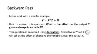
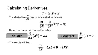
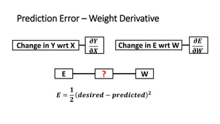
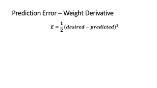
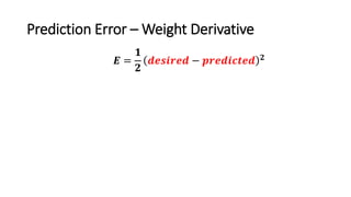
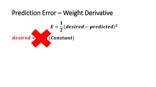
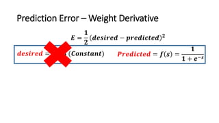
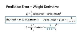
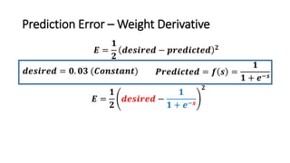
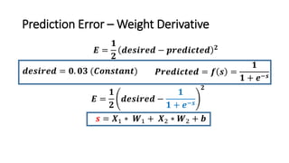
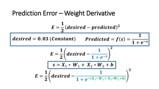
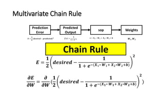
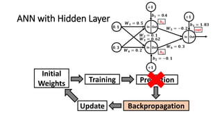
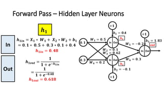
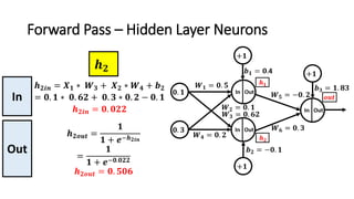
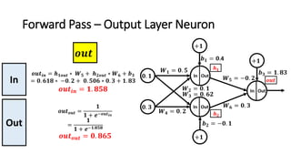

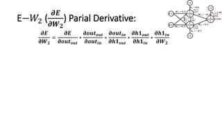
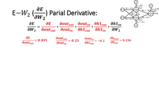
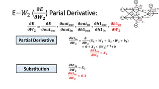
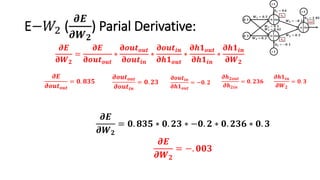
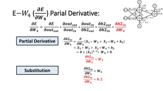
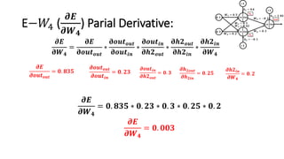
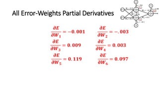
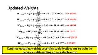

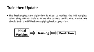
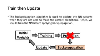
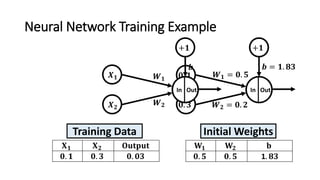
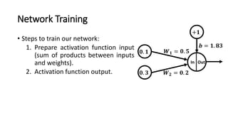
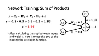
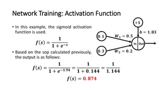
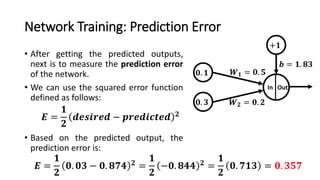
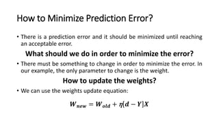
The document detailed the backpropagation algorithm used for updating weights in artificial neural networks (ANNs) to improve prediction accuracy. It explained the steps for training a neural network, calculating activation functions, predicting outputs, and minimizing prediction errors through weight updates. The importance of understanding how changes to weights affect errors in predictions was emphasized, along with the mathematical formulations involved in these processes.