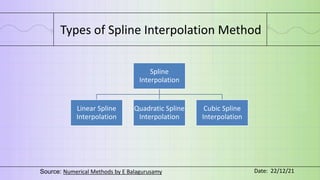
The document is a presentation on spline interpolation methods, covering definitions, types, algorithms, and examples. It explains linear and cubic spline interpolation, including their advantages and disadvantages, along with practical examples for better understanding. The conclusion emphasizes the efficiency and accuracy of spline interpolation compared to traditional polynomial interpolation.

1. Presentation on
Spline Interpolation Method
Presented By:
Shamim Ahammad Rasel (1805033)
Imran Islam (1805036)
Md. Wahid Ahmed Shanto (1805037)
Shahidul Ahad Sakib (1805038)
Md. Shohanur Islam ( 1805039)
Students,
Department of Computer Science
& Engineering,
Begum Rokeya University, Rangpur.
BEGUM ROKEYA UNIVERSITY, RANGPUR
Course Title: Numerical Methods Course Code: MAT 2221

2. MAIN TOPICS
POINTS TO TALK ABOUT
Definition
Why spline Interpolation?
Spline polynomial conditions
Example of spline polynomial
Types of Spline Polynomial Method
Linear Spline Interpolation
Cubic Spline Interpolation
Algorithm
Proof and example
Advantages, Disadvantages, Conclusion

3. Spline
Interpolation
PRESENTED BY :
SHAMIM AHMMAD RASEL
ID: 1805033

4. Definition
Spline interpolation is a form of interpolation where
the interpolant is a special type of piecewise
polynomial called spline.
It is also known as piecewise interpolation.
Source: google.com Date: 22/12/21

5. As it has been proved that when n is large
compared to the order of “true” function
the interpolation polynomial of degree n
does not provide accurate result at the end
of the range.
Why Spline Interpolation??
Source: Numerical Methods by E Balagurusamy Date: 22/12/21

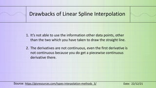
6. Spline polynomial conditions
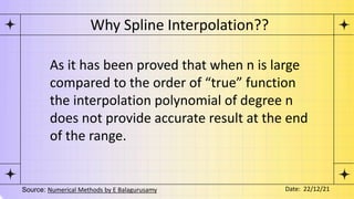
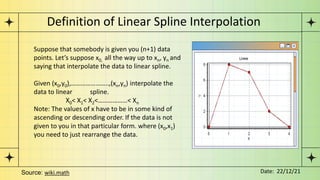
A spline function s(x) of degree m must satisfy the following
conditions
(i) s(x) is a polynomial of degree at most m in each of subinterval
[xi, xi+1] , I = 0,1,2 …. n.
(ii) S(x) and its derivatives of order 1,2…. m -1 are continuous in
the range [x0, xn].
Source: Numerical Methods by E Balagurusamy Date: 22/12/21

7. Example of piecewise Spline polynomial
f(x) =
𝑥 + 1 − 1 ≤ 𝑥 ≤ 0
2𝑥 + 1 0 ≤ 𝑥 ≤ 1
4 − 𝑥 1 ≤ 𝑥 ≤ 2
Here, n = 4 and x0 = -1, x1 = 0, x2 = 1, x3 x= 2
f1(x) = x + 1
f2(x) = 2x + 1
f3(x) = 4 - x
So, f1(x1) = 0 +1 = 1
f2(x1) = 2 x 0 +1 = 1
f2(x2) = 2 x 1 +1 = 3
f3(x2) = 4 -1 = 3
Here f1(x1) = f2(x1) and f2(x2) = f3(x2)
so piecewise are continuous and f(x) is spline.
Source: Numerical Methods by E Balagurusamy Date: 22/12/21

8. Linear Spline
Interpolation
PRESENTED BY :
WAHID AHMED SHANTO
ID: 1805037

9. Types of Spline Interpolation Method
Spline
Interpolation
Linear Spline
Interpolation
Quadratic Spline
Interpolation
Cubic Spline
Interpolation
Source: Numerical Methods by E Balagurusamy Date: 22/12/21

10. Definition of Linear Spline Interpolation
Suppose that somebody is given you (n+1) data
points. Let’s suppose x0, all the way up to xn, yn and
saying that interpolate the data to linear spline.
Given (x0,y0),…………………..,(xn,yn) interpolate the
data to linear spline.
X0< X1< X2<………………< Xn
Note: The values of x have to be in some kind of
ascending or descending order. If the data is not
given to you in that particular form. where (x0,x1)
you need to just rearrange the data.
Source: wiki.math Date: 22/12/21

11. Equation of Linear Spline Interpolation
f1(x) = yi +
𝑦𝑖+1 − 𝑦𝑖
𝑥𝑖+1− 𝑥𝑖
(x-xi) , { xi ≤ 𝑥 ≤ 𝑥𝑖+1}
f1(x) = y0 +
𝑦1 − 𝑦0
𝑥1− 𝑥0
(x-x0) , { x0 ≤ 𝑥 ≤ 𝑥1}
So what you are basically finding out is that the equations of the linear splines are
separate for each of the two consecutive data points as your seeing from there
things shown here. So that’s how linear spline works.
Linear spline works just like you linear interpolation the only thing is that you are
writing down the equations for every two consecutive data points, So as to be able
to write down the splines going from the first data point to the last data points, so
that’s what linear splines all about.
Source: wiki.math Date: 22/12/21

12. Drawbacks of Linear Spline Interpolation
1. It’s not able to use the information other data points, other
than the two which you have taken to draw the straight line.
2. The derivatives are not continuous, even the first derivative is
not continuous because you do get a piecewise continuous
derivative there.
Source: https://gisresources.com/types-interpolation-methods_3/ Date: 22/12/21

13. Example of Linear Spline Interpolation
Time(s) Velocity(m/s)
0 0
10 227.04
20 517.35
15 362.78
22.5 602.97
What the value of the velocity at 16 is by using linear spline
interpolation v(16)=?
Source: Numerical Methods by E Balagurusamy Date: 22/12/21

14. The data is not given in the right form.
So we will rearrange the data in ascending order.
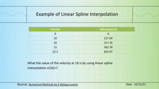
Time(s) Velocity(m/s)
0 0
10 227.04
15 362.78
20 517.35
22.5 602.97
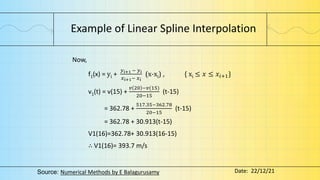
Now we have to find the value v(16)=?
So for that we are going to take[15,20] values because only this section is
bracket the value 16.
Example of Linear Spline Interpolation
Source: Numerical Methods by E Balagurusamy Date: 22/12/21

15. Example of Linear Spline Interpolation
Now,
f1(x) = yi +
𝑦𝑖+1 − 𝑦𝑖
𝑥𝑖+1− 𝑥𝑖
(x-xi) , { xi ≤ 𝑥 ≤ 𝑥𝑖+1}
v1(t) = v(15) +
𝑣 20 −𝑣(15)
20−15
(t-15)
= 362.78 +
517.35−362.78
20−15
(t-15)
= 362.78 + 30.913(t-15)
V1(16)=362.78+ 30.913(16-15)
∴ V1(16)= 393.7 m/s
Source: Numerical Methods by E Balagurusamy Date: 22/12/21

16. Cubic Spline
Interpolation
PRESENTED BY :
MD SHOHANUR ISLAM
ID: 1805039

17. Cubic Spline Interpolation
Consider a problem of interpolating between the following data points
using spline fitting.
X: x0 X1 X2 ……. Xn
Y: y0 y1 y2 …… yn
Assumptions of Cubic Spline S 𝑥 :
• S 𝑥 is a linear polynomial outside the interval (x0, xn).
• S 𝑥 is a cubic polynomial in each of the subintervals.
• S′ 𝑥 and S" 𝑥 are continuous at each point.
Now since S 𝑥 is a cubic in each subinterval so S” 𝑥 the
shall be linear.
Source: Youtube Video Date: 22/12/21

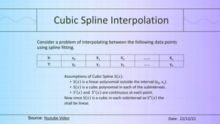
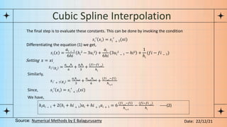
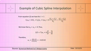
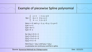
18. Cubic Spline Interpolation
Taking equally spaced values of x so that 𝑥𝑖 + 1 − 𝑥𝑖 = ℎ,
So according to Lagrange’s interpolation,
we can write:
𝑆" 𝑥 =
(𝑥−𝑥𝑖+1
)
(𝑥𝑖
−𝑥𝑖+1
)
𝑆" 𝑥𝑖 +
(𝑥−𝑥𝑖
)
(𝑥𝑖+1
−𝑥𝑖
)
𝑆" 𝑥𝑖 + 1
Integrating this equation twice, we have:
𝑠𝑖 𝑥 =
𝑎𝑖 − 1
6ℎ𝑖
ℎ𝑖
2𝑢𝑖 − 𝑢𝑖3 +
𝑎𝑖
6ℎ𝑖
𝑢𝑖
3
− 1 − ℎ𝑖2𝑢𝑖 − 1 +
1
ℎ𝑖
(𝑓𝑖𝑢𝑖 − 1 − 𝑓𝑖 − 1𝑢𝑖) −−−− −(1)
Source: Numerical Methods by E Balagurusamy Date: 22/12/21
Or 𝑆" 𝑥 =
(𝑥−𝑥𝑖+1
)
−ℎ
𝑆" 𝑥𝑖 +
(𝑥−𝑥𝑖
)
ℎ
𝑆" 𝑥𝑖 + 1
Or 𝑆" 𝑥 =
1
ℎ
𝑥𝑖 + 1 − 𝑥 𝑆"(𝑥𝑖) + (𝑥 − 𝑥𝑖)𝑆" 𝑥𝑖 ]

19. The final step is to evaluate these constants. This can be done by invoking the condition
𝑠𝑖
′
𝑥𝑖 = 𝑠𝑖
′
+ 1(𝑥𝑖)
Differentiating the equation (1) we get,
𝑠𝑖 𝑥 =
𝑎𝑖 − 1
6ℎ𝑖
ℎ𝑖
2 − 3𝑢𝑖
2 +
𝑎𝑖
6ℎ𝑖
3𝑢𝑖
2
− 1 − ℎ𝑖2 +
1
ℎ𝑖
(𝑓𝑖 − 𝑓𝑖 − 1)
Similarly,
𝑠𝑖
′
+ 1 𝑥𝑖
=
𝑎𝑖ℎ𝑖+1
3
+
𝑎𝑖+1ℎ𝑖+1
6
+
(𝑓𝑖+1−𝑓𝑖)
ℎ𝑖+1
Since, 𝑠𝑖
′
𝑥𝑖 = 𝑠𝑖
′
+ 1(𝑥𝑖)
ℎ𝑖𝑎𝑖 − 1 + 2 ℎ𝑖 + ℎ𝑖 + 1 𝑎𝑖 + ℎ𝑖 + 1𝑎𝑖 + 1 = 6
𝑓𝑖+1
−𝑓𝑖
ℎ𝑖+1
−
(𝑓𝑖−𝑓𝑖−1
)
ℎ𝑖
-----(2)
We have,
Cubic Spline Interpolation
Source: Numerical Methods by E Balagurusamy Date: 22/12/21
Setting 𝑥 = 𝑥𝑖,
𝑠𝑖
′
𝑥𝑖
=
𝑎𝑖−1ℎ𝑖
6
+
𝑎𝑖ℎ𝑖
3
+
(𝑓𝑖−𝑓𝑖−1)
ℎ𝑖

20. • When we write the all interior knots (i = 1,2, …..n-1), we get n-
1 simultaneous equations containing n+1 unknowns
(a0, a1, ,….. an).
Now applying the condition that the second derivatives at the
end point are zero, we get
a0 = an = 0
Cubic Spline Interpolation
Source: Numerical Methods by E Balagurusamy Date: 22/12/21

21. Example of
Cubic Spline Interpolation
PRESENTED BY :
SHAHIDUL AHAD SAKIB
ID: 1805038

22. Example of Cubic Spline Interpolation
Let us proceed with the help of an example bellow:
𝑖 0 1 2
𝑥𝑖 4 9 16
𝑓𝑖 2 3 4
Estimate the function value f at 𝑥 = 7 using cubic splines,
ℎ1 = 𝑥1 − 𝑥0 = 9 − 4 = 5
ℎ2 = 𝑥2 − 𝑥1 = 16 − 9 = 7
𝑓0 = 2, 𝑓1 = 3, 𝑓3 = 4
Source: Numerical Methods by E Balagurusamy Date: 22/12/21

23. Example of Cubic Spline Interpolation
From equation (2) we have for 𝑖 = 1
ℎ1𝑎0 + 2 ℎ1 + ℎ2 𝑎1 + ℎ2𝑎2 = 6
𝑓2 − 𝑓1
ℎ2
−
(𝑓1 − 𝑓0)
ℎ1
We know that 𝑎0 = 𝑎2 = 0. Thus,
2(5 + 7)𝑎1 = 6
1
7
−
1
5
Source: Numerical Methods by E Balagurusamy Date: 22/12/21
Therefore,
𝑎1 =
(6)(−2)
(35)(24)
= −0.0143

24. Example of Cubic Spline Interpolation
Since 𝑛 = 3, there are two cubic splines, namely
𝑠1 𝑥 𝑥0 ≤ 𝑥 ≤ 𝑥1
𝑠2 𝑥 𝑥1 ≤ 𝑥 ≤ 𝑥2
The target point 𝑥 = 7 is in the domain of 𝑠1(𝑥) and therefore. We need to use
only 𝑠 (𝑥) for estimation.
𝑢0 = 𝑥 − 𝑥0 and 𝑢1 = 𝑥 − 𝑥1
Source: Numerical Methods by E Balagurusamy Date: 22/12/21
From equation (1)
𝑠1 𝑥 =
𝑎0 𝑢0
3 − ℎ1
2𝑢0
6ℎ1
+
1
ℎ1
(𝑓1𝑢0 − 𝑓0𝑢1)

25. Example of Cubic Spline Interpolation
Upon substitution of specific values,
𝑠1 7 = −
0.0143
6 𝑋 5
7 − 4 3 − 52 7 − 4
= +
1
5
3 7 − 4 − 2 7 − 9
= 2.6229
Source: Numerical Methods by E Balagurusamy Date: 22/12/21

26. Advantage, Disadvantage &
Conclusion
PRESENTED BY :
MD IMRAN ISLAM
ID: 1805036

27. • Spline interpolation is useful for estimating above
maximum and below minimum points.
• It creates a smooth surface effect.
• Spline interpolation is a computationally efficient method
and the produced algorithm can easily be implemented on
a computer.
• Cubic splines has the ability to interpolate data with
smooth curves.
Advantages of Spline Interpolation
Source: https://gisresources.com/types-interpolation-methods_3/ Date: 22/12/21

28. • Cliffs and fault lines are not well presented because of the
smoothing effect.
• When the sample points are close together and have
extreme differences in value, spline interpolation doesn’t
work as well because spline uses slope calculation to
figure out the shape of the flexible rubber sheet.
Disadvantages of spline interpolation
Source: https://gisresources.com/types-interpolation-methods_3/ Date: 22/12/21

29. We have already known that, a spline is a special function
defined piecewise in polynomials. Spline interpolation is
often preferred to polynomial interpolation because it yields
similar results, even when using low degree polynomials.
The advantages of spline interpolation is higher accuracy
with less computational effort. This interpolation creates a
great efforts in numerical methods. By studying in this slide,
we should have good knowledge about spline interpolation.
Conclusion
Source: Google Date: 22/12/21

30. Thank You
For Your Attention!