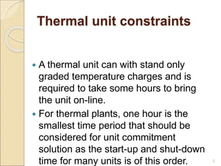
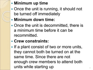
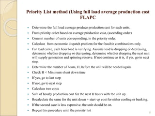
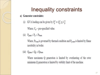
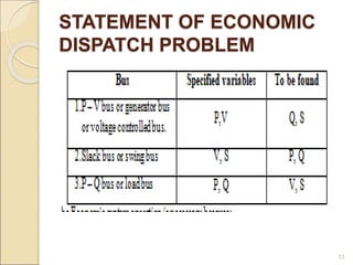
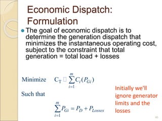
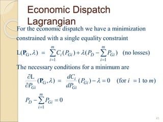
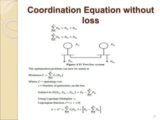
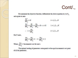
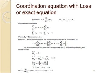
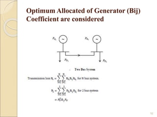
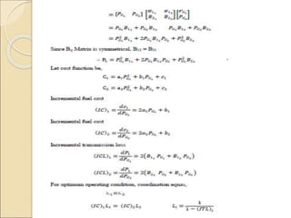
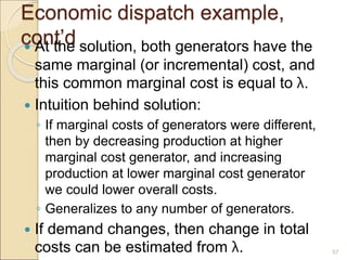
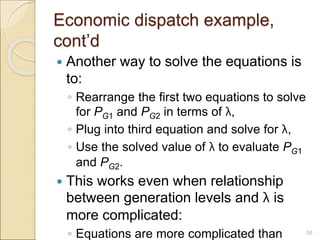
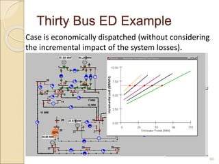
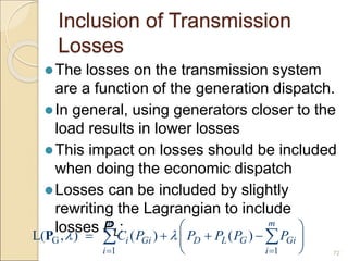
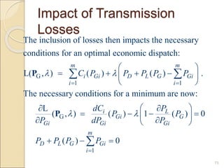
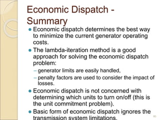
1) Thermal power plants have minimum up and down time constraints due to the time required to bring units online and cool them back down. One hour is typically the smallest time period considered for unit commitment. 2) Economic dispatch aims to minimize total operating costs given demand and transmission constraints. This is done by allocating generation across available units to equalize their marginal costs. 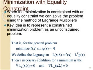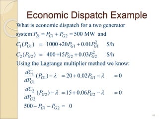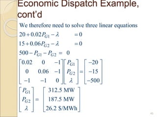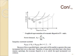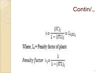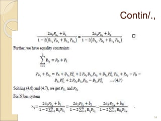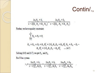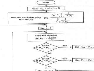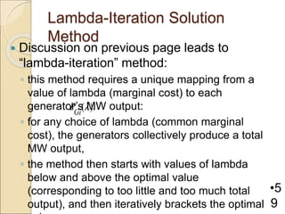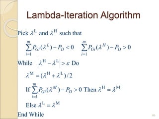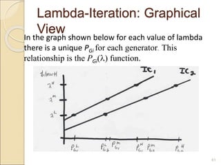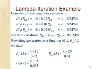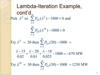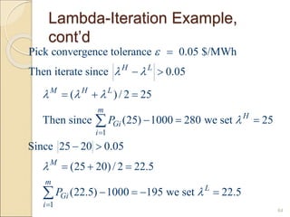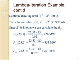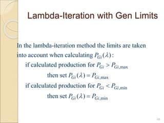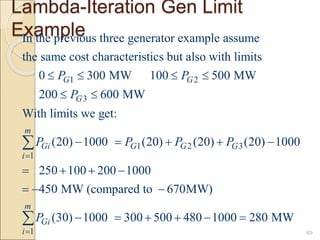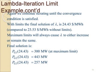3) The lambda-iteration method solves economic dispatch by iteratively choosing a system marginal cost (lambda) and calculating the corresponding generation dispatch until demand is met with minimum costs. It generalizes to systems with multiple non-linear generator cost functions.

1. UNIT-IV
UNIT COMMITMENT AND
ECONOMIC DISPATCH
1

2. Thermal unit constraints
 A thermal unit can with stand only
graded temperature charges and is
required to take some hours to bring
the unit on-line.
 For thermal plants, one hour is the
smallest time period that should be
considered for unit commitment
solution as the start-up and shut-down
time for many units is of this order. 2

3.  Minimum up time
 Once the unit is running, it should not
be turned off immediately
 Minimum down time:
 Once the unit is decommitted, there is
a minimum time before it can be
recommitted.
 Crew constraints:
 If a plant consist of two or more units,
they cannot both be turned on at the
same time. Since there are not
enough crew members to attend both
units while starting up 3

4.  Start-up cost:
 It is dependent upon the down-time of
the unit i.e., the time interval between
shut-down and restart.
 Start-up cost when cooling :
 During down time period, the unit’s
boiler to cool down and then heat back
up tp operating temperature in time for
a scheduled turn on
4

5. Start – up cost when banking
(shut-down cost)
 During shut-down period, the boiler
may be allowed to cool down and thus
no shut down cost will be incurred.
5

6. Hydro constraints
 In hydro-thermal scheduling, to
allocate maximum hydro units during
rainy seasons and to allocate thermal
units during remaining periods.
Fuel constraints:
If thermal and hydro sources are
available, a combined operation is
economic and advantageous i.e., to
minimize the fuel cost of thermal unit
over a commitment period.
6

7. Daily load curve
7

8. UNIT COMMITMENT
SOLUTION METHODS
 To form loading pattern for M –
Periods using load curve.
 • Commit possible number of units to
be operated to meet out the load.
 • To determine the load dispatch for all
feasible combination of solution for
each load level and satisfying
operating limits of each units.
8

9. Brute Force Technique or
Simple Priority List scheme
9

10. Peak – Valley” pattern
10
If the operation of the system is to be optimized, units must be shut down as
the load gets down and then recommitted as it goes back up

11. Priority List method (Using full load average production cost
FLAPC
 Determine the full load average produce production cast for each units.
 From priority order based on average production cost, (ascending order)
 Commit number of units corresponding, to the priority order.
 Calculate from economic dispatch problem for the feasible combinations only.
 For load curve, each hour load is verifying. Assume load is dropping or decreasing,
determine whether dropping or decreasing, determine whether dropping the next unit
will supply generation and spinning reserve. If not continue as it is, if yes, go to next
step.
 Determine the number of hours, H, before the unit will be needed again.
 Check H < Minimum shunt down time
 If yes, go to last step
 If not, go to next step
 Calculate two costs
 Sum of hourly production cost for the next H hours with the unit up.
 Recalculate the same for the unit down + start-up cost for either cooling or banking.
 If the second case is less expensive, the unit should be on.
 Repeat this procedure until the priority list
11

12. Dynamic Programming Method
12

13. STATEMENT OF ECONOMIC
DISPATCH PROBLEM
13

14. Necessity of economic
dispatch
 In many cases economic factor and the availability of priority essentials
such as coal, water etc. dictate that new generating plants is located at
greater distances from the load centers.
 The installation of larger blocks of power has resulted in the necessity of
transmitting power out of a given area until the load in that area is equal to
the new block of installed capacity.
 Power systems are inter connecting for purposes of economy interchange
and reduction of reserve capacity.
 In a number of areas of the country, the cost of fuel is rapidly increasing
14

15. Generation Strategy
15

16. Daily load curve
 Base load units
 Intermediate units
 Peaking units
 Reserve units
16

17. Base load units
 Nuclear units full under this category.
It is necessary to maintain the thermal
balance of the nuclear reactor and
steam system. Hence it is desirable to
maintain the megawatt output of such
units at a constants level.
17

18. Intermediate units
 Hydro powered units are best suited in
cases where the power output has to
be regulated. The output is controlled
by changing the water flow through
the turbine. In the absence of hydro
power thermal units has to be used
18

19. Peaking units
 In case of sudden increase in the load
the best choice is the gas – tubing
driving generators pumped hydro
storage and compressed gas are the
special type of peaking equipment
which can be used for this purpose
19

20. Reserve units:
Generators which are maintained at partial output and generators which are
ready for operation comes under this category
Problems involved:
 Hourly shifting of the power demand
 Generating unit must be regularly
maintained and, in case of nuclear units, it
must be refueled.
 Ability of the system to match the
generation to the load not only over the 24
hours daily time span but over seasons
and years
20

21. Economic Dispatch
 The purpose of economic dispatch or
optimal dispatch is to reduce fuel cost
for the power system. By economic
load scheduling, we mean to find the
generation of the different generations
of plants, so that the total fuel cost is
minimum and at the same time the
total demand and losses at any instant
must be met by the total generation
21

22. Methods
 Base load method: where the most
efficient unit is loaded to its maximum
capability, then the second most
efficient unit is loaded etc.
 Best point loading: (Incremental
method) where units are successively
loaded to their lowest heat rate point
beginning with the most efficient unit
and working down to the least efficient
unit.
22

23. 23

24. OPTIMAL OPERATION OF
GENERATORS ON A BUSBAR
 Generator Operating Cost :
 The total generator operating cost
includes fuel cost, cost of transmission
loss, labour and maintenance cost.
For simplicity, fuel, cost is considered
to be variable
24

25. Cost of generation depends on
operating constraints or system
constraints
 Equality constraint
 Inequality constraints
 Voltage constraints
 Running space capacity constraints
 Transformer tap settings
 Transmission line constraints
 Network securing
25

26. Equality constraint
26

27. Inequality constraints
27

28. Voltage constraints
28

29. Running and Transformer tap
29

30. Transmission line constraints
and
Network securing
30

31. Input – output characteristics
of a generating unit
31

32. HEAT RATE CURVE
32

33. 33
Incremental heat rate

34. Cost function
34

35. Incremental Cost Curve of Received Power (or)
System Incremental Cost (or) Incremental Fuel
Cost (IC) (or) Incremental Operating cost
35

36. Incremental fuel cost curve
36

37. Incremental cost curve for
thermal power plant
37

38. Input- output curve and incremental
cost curve for hydro power plant
38

39. Two Area System
39
Three possible cases are:
1. Area A is generating power at a lower incremental cost than area B and
possesses extra spinning reserve.
2. Area B will save money simply by purchasing extra MW from area A
which is generating power at a lower cost than area B.
3. Area A would benefit economically from selling power to area B as long as
area B is willing to pay a price.

40. Economic Dispatch:
Formulation
 The goal of economic dispatch is to
determine the generation dispatch that
minimizes the instantaneous operating cost,
subject to the constraint that total
generation = total load + losses
40
T
1
1
Minimize C ( )
Such that
m
i Gi
i
m
Gi D Losses
i
C P
P P P


 


Initially we'll
ignore generator
limits and the
losses

41. Unconstrained Minimization
 This is a minimization problem with a single equality
constraint
 For an unconstrained minimization a necessary (but
not sufficient) condition for a minimum is the gradient
of the function must be zero,
 The gradient generalizes the first derivative for multi-
variable problems:
41
1 2
( ) ( ) ( )
( ) , , ,
n
x x x
 
  
  
  
 
f x f x f x
f x
( )
 
f x 0

42. Minimization with Equality
Constraint
 When the minimization is constrained with an
equality constraint we can solve the problem
using the method of Lagrange Multipliers
 Key idea is to represent a constrained
minimization problem as an unconstrained
problem.
42
That is, for the general problem
minimize ( ) s.t. ( )
We define the Lagrangian L( , ) ( ) ( )
Then a necessary condition for a minimum is the
L ( , ) 0 and L ( , ) 0
T

 
   
x λ
f x g x 0
x λ f x λ g x
x λ x λ

43. Economic Dispatch
Lagrangian
43
G
1 1
G
For the economic dispatch we have a minimization
constrained with a single equality constraint
L( , ) ( ) ( ) (no losses)
The necessary conditions for a minimum are
L
( , )
m m
i Gi D Gi
i i
Gi
C P P P
dC
P
 

 
  



 
P
P
1
( ) 0 (for 1 to )
0
i
Gi
Gi
m
D Gi
i
P i m
dP
P P


  
 


44. Economic Dispatch Example
44
1 2
2
1 1 1 1
2
2 2 2 2
1
1
1
What is economic dispatch for a two generator
system 500 MW and
( ) 1000 20 0.01 $/h
( ) 400 15 0.03 $/h
Using the Lagrange multiplier method we know:
( ) 20 0.0
D G G
G G G
G G G
G
G
P P P
C P P P
C P P P
dC
P
dP

  
  
  
   1
2
2 2
2
1 2
2 0
( ) 15 0.06 0
500 0
G
G G
G
G G
P
dC
P P
dP
P P

 
 
    
  

45. Economic Dispatch Example,
cont’d
45
1
2
1 2
1
2
1
2
We therefore need to solve three linear equations
20 0.02 0
15 0.06 0
500 0
0.02 0 1 20
0 0.06 1 15
1 1 0 500
312.5 MW
187.5 MW
26.2 $/MW
G
G
G G
G
G
G
G
P
P
P P
P
P
P
P




  
  
  
 
    
    
  
    
  
    
    
 
  
 
 
  h
 
 
 
 
 

46. Inequality constraints
46

47. Coordination Equation without
loss
47

48. Cont/.,
48

49. Con/.,
49

50. Coordination equation with Loss
or exact equation
50

51. Contin/.,
51

52. Optimum Allocated of Generator (Bij)
Coefficient are considered
52

53. Contin/.,
53

54. Contin/.,
54

55. Contin/.,
55

56. 56

57. Economic dispatch example,
cont’d
 At the solution, both generators have the
same marginal (or incremental) cost, and
this common marginal cost is equal to λ.
 Intuition behind solution:
◦ If marginal costs of generators were different,
then by decreasing production at higher
marginal cost generator, and increasing
production at lower marginal cost generator
we could lower overall costs.
◦ Generalizes to any number of generators.
 If demand changes, then change in total
costs can be estimated from λ. 57

58. Economic dispatch example,
cont’d
 Another way to solve the equations is
to:
◦ Rearrange the first two equations to solve
for PG1 and PG2 in terms of λ,
◦ Plug into third equation and solve for λ,
◦ Use the solved value of λ to evaluate PG1
and PG2.
 This works even when relationship
between generation levels and λ is
more complicated:
◦ Equations are more complicated than 58

59. Lambda-Iteration Solution
Method
 Discussion on previous page leads to
“lambda-iteration” method:
◦ this method requires a unique mapping from a
value of lambda (marginal cost) to each
generator’s MW output:
◦ for any choice of lambda (common marginal
cost), the generators collectively produce a total
MW output,
◦ the method then starts with values of lambda
below and above the optimal value
(corresponding to too little and too much total
output), and then iteratively brackets the optimal
•5
9
( ).
Gi
P 

60. Lambda-Iteration Algorithm
60
L H
1 1
H L
M H L
H M
1
L M
Pick and such that
( ) 0 ( ) 0
While Do
( )/2
If ( ) 0 Then
Else
End While
m m
L H
Gi D Gi D
i i
m
M
Gi D
i
P P P P
P P
 
 
  
  
  
 
 

   
 
 
  

 


61. Lambda-Iteration: Graphical
View
61
In the graph shown below for each value of lambda
there is a unique PGi for each generator. This
relationship is the PGi() function.

62. Lambda-Iteration Example
62
1 1 1
2 2 2
3 3 3
1 2 3
Consider a three generator system with
( ) 15 0.02 $/MWh
( ) 20 0.01 $/MWh
( ) 18 0.025 $/MWh
and with constraint 1000MW
Rewriting generation as a function of , (
G G
G G
G G
G G G
Gi
IC P P
IC P P
IC P P
P P P
P




  
  
  
  
1 2
3
),
we have
15 20
( ) ( )
0.02 0.01
18
( )
0.025
G G
G
P P
P

 
 


 
 



63. Lambda-Iteration Example,
cont’d
63
m
i=1
m
i=1
1
H
1
Pick so ( ) 1000 0 and
( ) 1000 0
Try 20 then (20) 1000
15 20 18
1000 670 MW
0.02 0.01 0.025
Try 30 then (30) 1000 1230 MW
L L
Gi
H
Gi
m
L
Gi
i
m
Gi
i
P
P
P
P
 


  



 
 
  
  
    
  





64. Lambda-Iteration Example,
cont’d
64
1
1
Pick convergence tolerance 0.05 $/MWh
Then iterate since 0.05
( )/ 2 25
Then since (25) 1000 280 we set 25
Since 25 20 0.05
(25 20)/ 2 22.5
(22.5) 1000 195 we set 2
H L
M H L
m
H
Gi
i
M
m
L
Gi
i
P
P

 
  






 
  
  
 
  
   

 2.5

65. Lambda-Iteration Example,
cont’d
65
H
*
*
1
2
3
Continue iterating until 0.05
The solution value of , , is 23.53 $/MWh
Once is known we can calculate the
23.53 15
(23.5) 426 MW
0.02
23.53 20
(23.5) 353 MW
0.01
23.53 18
(23.5)
0.025
L
Gi
G
G
G
P
P
P
P
 
 

 

 

 

 221 MW


66. Thirty Bus ED Example
66
Case is economically dispatched (without considering
the incremental impact of the system losses).

67. Generator MW Limits
Generators have limits on the minimum
and maximum amount of power they can
produce
Typically the minimum limit is not zero.
Because of varying system economics
usually many generators in a system are
operated at their maximum MW limits:
Baseload generators are at their maximum
limits except during the off-peak.
67

68. Lambda-Iteration with Gen Limits
68
,max
,max
In the lambda-iteration method the limits are taken
into account when calculating ( ) :
if calculated production for
then set ( )
if calculated production for
Gi
Gi Gi
Gi Gi
P
P P
P P




,min
,min
then set ( )
Gi Gi
Gi Gi
P P
P P




69. Lambda-Iteration Gen Limit
Example
69
1 2
3
1 2 3
1
In the previous three generator example assume
the same cost characteristics but also with limits
0 300 MW 100 500 MW
200 600 MW
With limits we get:
(20) 1000 (20) (20) (20) 10
G G
G
m
Gi G G G
i
P P
P
P P P P

   
 
    

1
00
250 100 200 1000
450 MW (compared to 670MW)
(30) 1000 300 500 480 1000 280 MW
m
Gi
i
P

   
  
     


70. Lambda-Iteration Limit
Example,cont’d
70
Again we continue iterating until the convergence
condition is satisfied.
With limits the final solution of , is 24.43 $/MWh
(compared to 23.53 $/MWh without limits).
Maximum limits will always caus

1
2
3
e to either increase
or remain the same.
Final solution is:
(24.43) 300 MW (at maximum limit)
(24.43) 443 MW
(24.43) 257 MW
G
G
G
P
P
P





71. Back of Envelope Values
 $/MWhr = fuelcost * heatrate + variable O&M
 Typical incremental costs can be roughly
approximated:
– Typical heatrate for a coal plant is 10, modern
combustion turbine is 10, combined cycle plant is
6 to 8, older combustion turbine 15.
– Fuel costs ($/MBtu) are quite variable, with current
values around 2 for coal, 3 to 5 for natural gas, 0.5
for nuclear, probably 10 for fuel oil.
– Hydro costs tend to be quite low, but are fuel
(water) constrained
– Wind and solar costs are zero.
71

72. Inclusion of Transmission
Losses
The losses on the transmission system
are a function of the generation dispatch.
In general, using generators closer to the
load results in lower losses
This impact on losses should be included
when doing the economic dispatch
Losses can be included by slightly
rewriting the Lagrangian to include
losses PL:
72
G
1 1
L( , ) ( ) ( )
m m
i Gi D L G Gi
i i
C P P P P P
 
 
 
   
 
 
 
P

73. Impact of Transmission
Losses
73
G
1 1
G
The inclusion of losses then impacts the necessary
conditions for an optimal economic dispatch:
L( , ) ( ) ( ) .
The necessary conditions for a minimum are now:
L
(
m m
i Gi D L G Gi
i i
Gi
C P P P P P
P
 
 
 
   
 
 


 
P
P
1
, ) ( ) 1 ( ) 0
( ) 0
i L
Gi G
Gi Gi
m
D L G Gi
i
dC P
P P
dP P
P P P P
 

 

   
 

 
  


74. Impact of Transmission
Losses
74
th
Solving for , we get: ( ) 1 ( ) 0
1
( )
1 ( )
Define the penalty factor for the generator
(don't confuse with Lagrangian L!!!)
1
1 ( )
i L
Gi G
Gi Gi
i
Gi
Gi
L
G
Gi
i
i
L
G
Gi
dC P
P P
dP P
dC
P
dP
P
P
P
L i
L
P
P
P
 

 

  
 

 

 


 

 

 

 




The penalty factor
at the slack bus is
always unity!

75. Impact of Transmission
Losses
75
1 1 1 2 2 2
The condition for optimal dispatch with losses is then
( ) ( ) ( )
1
. So, if increasing increases
1 ( )
the losses then ( ) 0 1.0
This makes generator
G G m m Gm
i Gi
L
G
Gi
L
G i
Gi
L IC P L IC P L IC P
L P
P
P
P
P
P L
P

  

 


 

 

  

appear to be more expensive
(i.e., it is penalized). Likewise 1.0 makes a generator
appear less expensive.
i
i
L 

76. Calculation of Penalty Factors
76
Unfortunately, the analytic calculation of is
somewhat involved. The problem is a small change
in the generation at impacts the flows and hence
the losses throughout the entire system. However,
i
Gi
L
P
using a power flow you can approximate this function
by making a small change to and then seeing how
the losses change:
1
( )
1
Gi
L L
G i
L
Gi Gi
Gi
P
P P
P L
P
P P
P
 
 

  


77. Two Bus Penalty Factor
Example
77
2 2
2 2
0.37
( ) 0.0387 0.037
10
0.9627 0.9643
L L
G
G G
P P MW
P
P P MW
L L
  
    
 
 

78. Thirty Bus ED Example
78
Now consider losses.
Because of the penalty factors the generator incremental
costs are no longer identical.

79. Area Supply Curve
79
0 100 200 300 400
Total Area Generation (MW)
0.00
2.50
5.00
7.50
10.00
The area supply curve shows the cost to produce the
next MW of electricity, assuming area is economically
dispatched
Supply
curve for
thirty bus
system

80. Economic Dispatch -
Summary
 Economic dispatch determines the best way
to minimize the current generator operating
costs.
 The lambda-iteration method is a good
approach for solving the economic dispatch
problem:
– generator limits are easily handled,
– penalty factors are used to consider the impact of
losses.
 Economic dispatch is not concerned with
determining which units to turn on/off (this is
the unit commitment problem).
 Basic form of economic dispatch ignores the
80

81. Security Constrained ED
or Optimal Power Flow
Transmission constraints often limit ability to
use lower cost power.
Such limits require deviations from what
would otherwise be minimum cost dispatch
in order to maintain system “security.”
Need to solve or approximate power flow in
order to consider transmission constraints.
81

82. Security Constrained ED
or Optimal Power Flow
The goal of a security constrained ED or
optimal power flow (OPF) is to determine
the “best” way to instantaneously operate
a power system, considering transmission
limits.
Usually “best” = minimizing operating cost,
while keeping flows on transmission below
limits.
In three bus case the generation at bus 3
must be limited to avoid overloading the
82

83. Security Constrained
Dispatch
Bus 2 Bus 1
Bus 3
Home Area
Scheduled Transactions
357 MW
179 MVR
194 MW
448 MW
19 MVR
232 MVR
179 MW
89 MVR
1.00 PU
-22 MW
4 MVR
22 MW
-4 MVR
-142 MW
49 MVR
145 MW
-37 MVR
124 MW
-33 MVR
-122 MW
41 MVR
1.00 PU
1.00 PU
0 MW
37 MVR
100%
100%
100 MW
OFF AGC
AVR ON
AGC ON
AVR ON
100.0 MW
83
Need to dispatch to keep line
from bus 3 to bus 2 from overloading

84. Multi-Area Operation
 In multi-area system, “rules” have been established
regarding transactions on tie-lines:
– In Eastern interconnection, in principle, up to “nominal”
thermal interconnection capacity,
– In Western interconnection there are more complicated
rules
 The actual power that flows through the entire
network depends on the impedance of the
transmission lines, and ultimately determine what
are acceptable patterns of dispatch:
Can result in need to “curtail” transactions that
otherwise satisfy rules.
 Economically uncompensated flow through other
areas is known as “parallel path” or “loop flows.”
 Since ERCOT is one area, all of the flows on AC
lines are inside ERCOT and there is no
uncompensated flow on AC lines.
84

85. Seven Bus Case: One-line
Top Area Cost
Left Area Cost Right Area Cost
1
2
3 4
5
6 7
106 MW
168 MW
200 MW 201 MW
110 MW
40 MVR
80 MW
30 MVR
130 MW
40 MVR
40 MW
20 MVR
1.00 PU
1.01 PU
1.04 PU
1.04 PU
1.04 PU
0.99 PU
1.05 PU
62 MW
-61 MW
44 MW -42 MW -31 MW 31 MW
38 MW
-37 MW
79 MW -77 MW
-32 MW
32 MW
-14 MW
-39 MW
40 MW
-20 MW
20 MW
40 MW
-40 MW
94 MW
200 MW
0 MVR
200 MW
0 MVR
20 MW -20 MW
AGC ON
AGC ON
AGC ON
AGC ON
AGC ON
8029 $/MWH
4715 $/MWH
4189 $/MWH
Case Hourly Cost
16933 $/MWH
85
System has
three areas
Left area
has one
bus
Right area has one
bus
Top area
has five
buses
No net
interchange
between
Any areas.

86. Seven Bus Case: Area View
Area Losses
Area Losses Area Losses
Top
Left Right
-40.1 MW
0.0 MW
0.0 MW
0.0 MW
40.1 MW
40.1 MW
7.09 MW
0.33 MW 0.65 MW
86
System has
40 MW of
“Loop Flow”
Actual
flow
between
areas
Loop flow can result in higher losses
Scheduled
flow

87. Seven Bus - Loop Flow?
Area Losses
Area Losses Area Losses
Top
Left Right
-4.8 MW
0.0 MW
100.0 MW
0.0 MW
104.8 MW
4.8 MW
9.44 MW
-0.00 MW 4.34 MW
87
100 MW Transaction
between Left and Right
Transaction has
actually decreased
the loop flow
Note that
Top’s
Losses have
increased
from
7.09MW to
9.44 MW