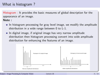
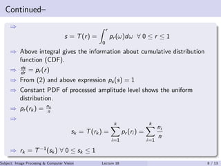
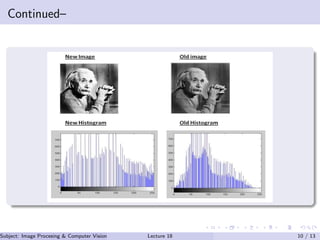
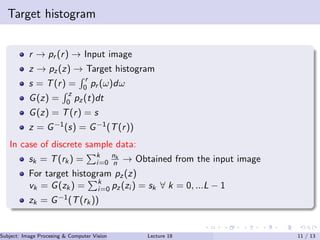
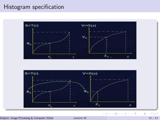
This document discusses histogram operations in image processing. It defines a histogram as providing a global description of an image's appearance by measuring the distribution of pixel intensities. Histogram equalization aims to create a uniform distribution of intensities by mapping values to enhance contrast. Histogram specification allows mapping pixel intensities from an input image to match a target histogram distribution to modify image characteristics. These histogram techniques are useful for improving features in images with narrow or uneven intensity distributions.

1. Histogram Operation in Image Processing
Subject: Image Procesing & Computer Vision
Dr. Varun Kumar
Subject: Image Procesing & Computer Vision Dr. Varun Kumar (.)Lecture 18 1 / 13

2. Outlines
1 What is Histogram ?
2 Histogram Equalization
3 Histogram Specification
4 References
Subject: Image Procesing & Computer Vision Dr. Varun Kumar (.)Lecture 18 2 / 13

3. What is histogram ?
Histogram : It provides the basic measures of global description for the
appearance of an image.
Note :
In histogram processing for gray level image, we modify the amplitude
distribution in a wide range between 0 to L-1.
In digital image, if original image has very narrow amplitude
distribution then histogram processing convert into wide amplitude
distribution for enhancing the features of an image.
Subject: Image Procesing & Computer Vision Dr. Varun Kumar (.)Lecture 18 3 / 13

4. Mathematical analysis of histogram plot
Let rk is the amplitude level of kth level. ∀ 0 ≤ k ≤ L − 1
h(rk) = nk
⇒ nk is the total number of pixels having amplitude level same as rk.
Normalized histogram :
p(rk) =
nk
n
(1)
⇒ Total number of available pixels in an image.
⇒ p(rk) denotes the probability of occurrence having amplitude level of
an image is equal to rk
Subject: Image Procesing & Computer Vision Dr. Varun Kumar (.)Lecture 18 4 / 13

5. Histogram image analysis
Dark image
Bright image
Subject: Image Procesing & Computer Vision Dr. Varun Kumar (.)Lecture 18 5 / 13

6. Continued–
Low contrast image
High contrast image
Subject: Image Procesing & Computer Vision Dr. Varun Kumar (.)Lecture 18 6 / 13

7. Histogram equalization
⇒ r represents gray level in an image.
⇒ General relation between original and processed amplitude value
s = T(r)
⇒ T(r) is single valued and monotonically increasing in 0 ≤ r ≤ 1
⇒ 0 ≤ T(r) ≤ 1 for 0 ≤ r ≤ 1
⇒ r = T−1(s) → Inversion process
⇒ Let pr (r) is the PDF of amplitude level r.
⇒ Similarly, ps(s) is the PDF of amplitude level s.
⇒ pr (r) and T(r) are known.
⇒ T−1(s) is monotonically increasing.
⇒ Also,
ps(s) = pr (r)|
ds
dr
|r=T−1(s) (2)
Subject: Image Procesing & Computer Vision Dr. Varun Kumar (.)Lecture 18 7 / 13

8. Continued–
⇒
s = T(r) =
r
0
pr (ω)dω ∀ 0 ≤ r ≤ 1
⇒ Above integral gives the information about cumulative distribution
function (CDF).
⇒ ds
dr = pr (r)
⇒ From (2) and above expression ps(s) = 1
⇒ Constant PDF of processed amplitude level shows the uniform
distribution.
⇒ pr (rk) = nk
n
⇒
sk = T(rk) =
k
i=1
pr (ri ) =
k
i=1
ni
n
⇒ rk = T−1(sk) ∀ 0 ≤ sk ≤ 1
Subject: Image Procesing & Computer Vision Dr. Varun Kumar (.)Lecture 18 8 / 13

9. Image equalization
Image equalization
Subject: Image Procesing & Computer Vision Dr. Varun Kumar (.)Lecture 18 9 / 13

10. Continued–
Subject: Image Procesing & Computer Vision Dr. Varun Kumar (.)Lecture 18 10 / 13

11. Target histogram
r → pr (r) → Input image
z → pz(z) → Target histogram
s = T(r) =
r
0 pr (ω)dω
G(z) =
z
0 pz(t)dt
G(z) = T(r) = s
z = G−1(s) = G−1(T(r))
In case of discrete sample data:
sk = T(rk) = k
i=0
nk
n → Obtained from the input image
For target histogram pz(z)
vk = G(zk) = k
i=0 pz(zi ) = sk ∀ k = 0, ...L − 1
zk = G−1(T(rk))
Subject: Image Procesing & Computer Vision Dr. Varun Kumar (.)Lecture 18 11 / 13

12. Histogram specification
Subject: Image Procesing & Computer Vision Dr. Varun Kumar (.)Lecture 18 12 / 13

13. References
M. Sonka, V. Hlavac, and R. Boyle, Image processing, analysis, and machine vision.
Cengage Learning, 2014.
D. A. Forsyth and J. Ponce, “A modern approach,” Computer vision: a modern
approach, vol. 17, pp. 21–48, 2003.
L. Shapiro and G. Stockman, “Computer vision prentice hall,” Inc., New Jersey,
2001.
R. C. Gonzalez, R. E. Woods, and S. L. Eddins, Digital image processing using
MATLAB. Pearson Education India, 2004.
Subject: Image Procesing & Computer Vision Dr. Varun Kumar (.)Lecture 18 13 / 13