Image enhancement for the image improvement

1. Digital Image
Processing
Image Enhancement
Histogram Processing
Instructor Name
Dr. Muhammad Sharif

2. Material Reference
2
Images and Material
From
Rafael C. Gonzalez and Richard E. Wood,
Digital Image Processing, 2nd
Edition.& Internet Resources

3. Contents
Over the next few lectures we will look at image
enhancement techniques working in the spatial
domain:
 Recap
 Different kinds of image enhancement
 Histograms
 Histogram equalization
3

4. A Note About Grey Levels
 So far when we have spoken about image grey level
values, we have said they are in the range [0, 255]
- Where 0 is black and 255 is white
 There is no reason why we have to use this range
- The range [0,255] stems from display technologies
 For many of the image processing operations in
this lecture grey levels are assumed to be given in
the range [0.0, 1.0]
4

5. What Is Image Enhancement?
Image enhancement is the process of making
images more useful
The reasons for doing this include:
 Highlighting interesting detail in images
 Removing noise from images
 Making images more visually appealing
5

6. Image Enhancement Examples
6

7. Image Enhancement Examples (cont.…)
7

8. Image Enhancement Examples (cont.…)
8

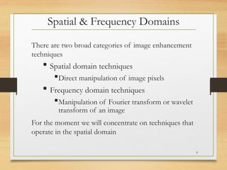
9. Spatial & Frequency Domains
There are two broad categories of image enhancement
techniques
 Spatial domain techniques
Direct manipulation of image pixels
 Frequency domain techniques
Manipulation of Fourier transform or wavelet
transform of an image
For the moment we will concentrate on techniques that
operate in the spatial domain
9

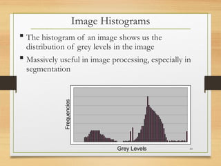
10. Image Histograms
 The histogram of an image shows us the
distribution of grey levels in the image
 Massively useful in image processing, especially in
segmentation
Grey Levels
Frequencies
10

11. Histogram Examples
11

12. Histogram Examples (cont.…)
12

13. Histogram Examples (cont.…)

14. Histogram Examples (cont.…)
14

15. Histogram Examples (cont.…)
15

16. Histogram Examples (cont.…)
16

17. Histogram Examples (cont.…)
17

18. Histogram Examples (cont…)
18

19. Histogram Examples (cont.…)
19

20. Histogram Examples (cont.…)
20

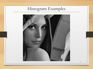
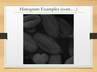
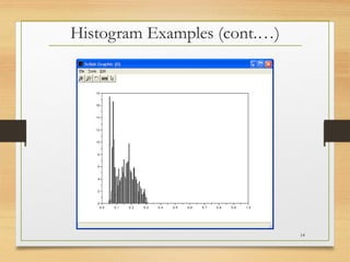
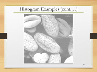
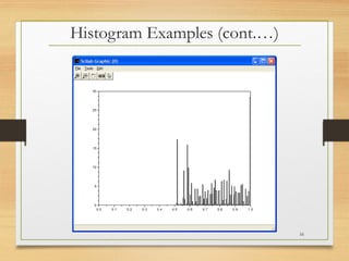
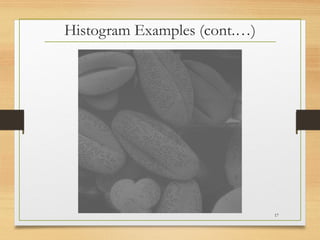
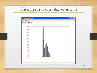
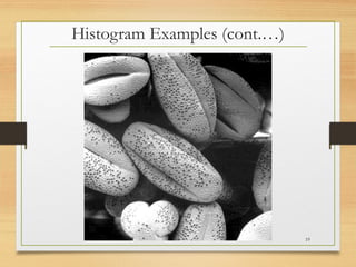
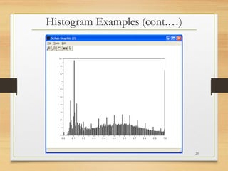
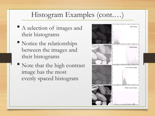
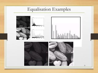
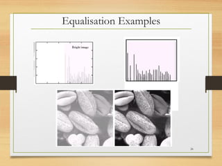
21. Histogram Examples (cont.…)
 A selection of images and
their histograms
 Notice the relationships
between the images and
their histograms
 Note that the high contrast
image has the most
evenly spaced histogram
21

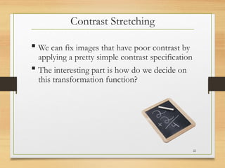
22. Contrast Stretching
 We can fix images that have poor contrast by
applying a pretty simple contrast specification
 The interesting part is how do we decide on
this transformation function?
22

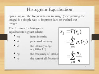
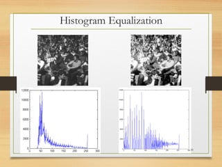
23. Histogram Equalisation
Spreading out the frequencies in an image (or equalising the
image) is a simple way to improve dark or washed out
images
The formula for histogram
equalisation is given where
 rk: input intensity
 sk: processed intensity
 k: the intensity range
(e.g 0.0 – 1.0)
 nj: the frequency of intensity j
 n: the sum of all frequencies
)
( k
k r
T
s 



k
j
j
r r
p
1
)
(



k
j
j
n
n
1
23

24. Equalisation Transformation Function
24

25. Equalisation Examples
25

26. Equalisation Examples
26

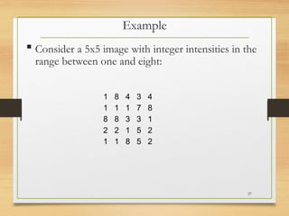
27.  Consider a 5x5 image with integer intensities in the
range between one and eight:
Example
1 8 4 3 4
1 1 1 7 8
8 8 3 3 1
2 2 1 5 2
1 1 8 5 2
27

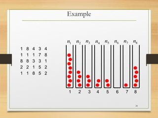
28. Example
1 8 4 3 4
1 1 1 7 8
8 8 3 3 1
2 2 1 5 2
1 1 8 5 2
1 2 3 4 5 6 7 8
1
n 2
n 3
n 4
n 5
n 6
n 7
n 8
n
28

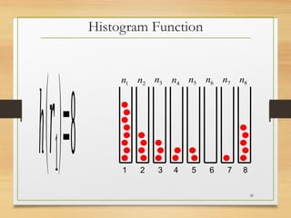
29. 1 2 3 4 5 6 7 8
1
n 2
n 3
n 4
n 5
n 6
n 7
n 8
n
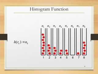
k
k n
r
h 
)
(
Histogram Function
29

30. h(𝑟1)=8 1 2 3 4 5 6 7 8
1
n 2
n 3
n 4
n 5
n 6
n 7
n 8
n
Histogram Function
30

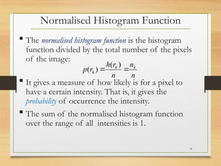
31.  The normalised histogram function is the histogram
function divided by the total number of the pixels
of the image:
 It gives a measure of how likely is for a pixel to
have a certain intensity. That is, it gives the
probability of occurrence the intensity.
 The sum of the normalised histogram function
over the range of all intensities is 1.
n
n
n
r
h
r
p k
k
k 

)
(
)
(
Normalised Histogram Function
31

32. Normalised Histogram Function
20
.
0
25
/
5
)
(
04
.
0
25
/
1
)
(
00
.
0
25
/
0
)
(
08
.
0
25
/
2
)
(
08
.
0
25
/
3
)
(
12
.
0
25
/
3
)
(
16
.
0
25
/
4
)
(
32
.
0
25
/
8
)
(
8
7
6
5
4
3
2
1
















r
p
r
p
r
p
r
p
r
p
r
p
r
p
r
p
5
)
(
1
)
(
0
)
(
2
)
(
2
)
(
3
)
(
4
)
(
8
)
(
8
7
6
5
4
3
2
1








r
h
r
h
r
h
r
h
r
h
r
h
r
h
r
h
32

33. Histogram Equalization
20
.
0
)
(
04
.
0
)
(
00
.
0
)
(
08
.
0
)
(
08
.
0
)
(
12
.
0
)
(
16
.
0
)
(
32
.
0
)
(
8
7
6
5
4
3
2
1








r
p
r
p
r
p
r
p
r
p
r
p
r
p
r
p

















)
(
)
(
)
(
)
(
68
.
0
08
.
0
12
.
0
16
.
0
32
.
0
)
(
60
.
0
12
.
0
16
.
0
32
.
0
)
(
48
.
0
16
.
0
32
.
0
)
(
32
.
0
)
(
8
7
6
5
4
3
2
1
r
T
r
T
r
T
r
T
r
T
r
T
r
T
r
T
Intensity transformation
function
Normalised
histogram function
33

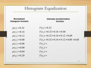
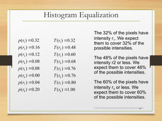
34. The 32% of the pixels have
intensity r1. We expect
them to cover 32% of the
possible intensities.
The 48% of the pixels have
intensity r2 or less. We
expect them to cover 48%
of the possible intensities.
The 60% of the pixels have
intensity r3 or less. We
expect them to cover 60%
of the possible intensities.
……………………………
00
.
1
)
(
80
.
0
)
(
76
.
0
)
(
76
.
0
)
(
68
.
0
)
(
60
.
0
)
(
48
.
0
)
(
32
.
0
)
(
8
7
6
5
4
3
2
1








r
T
r
T
r
T
r
T
r
T
r
T
r
T
r
T
20
.
0
)
(
04
.
0
)
(
00
.
0
)
(
08
.
0
)
(
08
.
0
)
(
12
.
0
)
(
16
.
0
)
(
32
.
0
)
(
8
7
6
5
4
3
2
1








r
p
r
p
r
p
r
p
r
p
r
p
r
p
r
p
Histogram Equalization
34

35. Histogram Equalization
35

36. Summary
We have looked at:
 Different kinds of image enhancement
 Histograms
 Histogram equalisation
Next time we will start to look at point processing
and some neighbourhood operations
36

37.  What is point processing?
 Negative images
 Thresholding
 Logarithmic transformation
 Power law transforms
 Grey level slicing
 Bit plane slicing
Next Lecture
37

38. 38
THANK YOU