KL Transform in Image Processing

1. KL Transform
Subject: Image Procesing & Computer Vision
Dr. Varun Kumar
Subject: Image Procesing & Computer Vision Dr. Varun Kumar (IIIT Surat)Lecture 16 1 / 10

2. Outlines
1 Introduction to KL transform
2 Fundamental difference between KL and other transform
3 Properties of KL transform
4 Computation of KL transform for an image
5 References
Subject: Image Procesing & Computer Vision Dr. Varun Kumar (IIIT Surat)Lecture 16 2 / 10

3. Introduction to KL transform
In another transform, like DFT, DCT, etc the transformation kernel are
fixed. Ex-
g(x, u) = e−2π
N
ux
⇒ In KL transformation, kernel are derived from the data, it does not
remain fixed.
⇒ It depends on the statistic (data treated as a random variable) rather
than deterministic.
⇒ In KL transformation data is represented into a vector representation.
Let a data population is represented as
X =





x1
x2
...
xn





⇒ µx = E(x) and Cx = E{(X − µx )(X − µx )T
}
Subject: Image Procesing & Computer Vision Dr. Varun Kumar (IIIT Surat)Lecture 16 3 / 10

4. Continued–
Note:
Here, µx is a vector of size n × 1, whereas Cx is matrix of size n × n.
Covariance matrix, Cx is real and symmetric.
Let ei is the eigen vector having λi entry.
Eigen values are arranged into descending order, i.e λj ≥ λj+1
Let a transformation matrix A is such a way that
y = A(X − µx ) where A ⇒ n × n matrix
Properties of y
1 Mean should be equal to zero, i.e E(y) = µy = 0.
2 Covariance matrix Cy = ACx AT .
Subject: Image Procesing & Computer Vision Dr. Varun Kumar (IIIT Surat)Lecture 16 4 / 10

5. Continued–
3 Here,
Cy =





λ1, 0 0 0 0 0
0 λ2, 0 0 0 0
...
...
...
...
...
0 0 0 0 0 λn





⇒ Off diagonal terms are zero ⇒ Each element of vector y is
statistically un-correlated from the remaining elements.
Implication :
Subject: Image Procesing & Computer Vision Dr. Varun Kumar (IIIT Surat)Lecture 16 5 / 10

6. Continued–
From above figure, the object is populated at the location (4,5), (5,5),
(6,5), (5,6), (6,6), (7,6), (5,7) and (6,7). Hence
X =
4
5
,
5
5
,
6
5
,
5
6
,
6
6
,
7
6
,
5
7
,
6
7
(1)
and
µx =
5.5
5.875
(2)
and
Cx = E{(x − µx )(x − µx )T
} =
6 1.5
1.5 4.875
(3)
For finding the eigen value of the covariance matrix
|Cx − λI2| = 0 ⇒ λ1 = 7.0395 λ2 = 3.8355 (4)
Subject: Image Procesing & Computer Vision Dr. Varun Kumar (IIIT Surat)Lecture 16 6 / 10

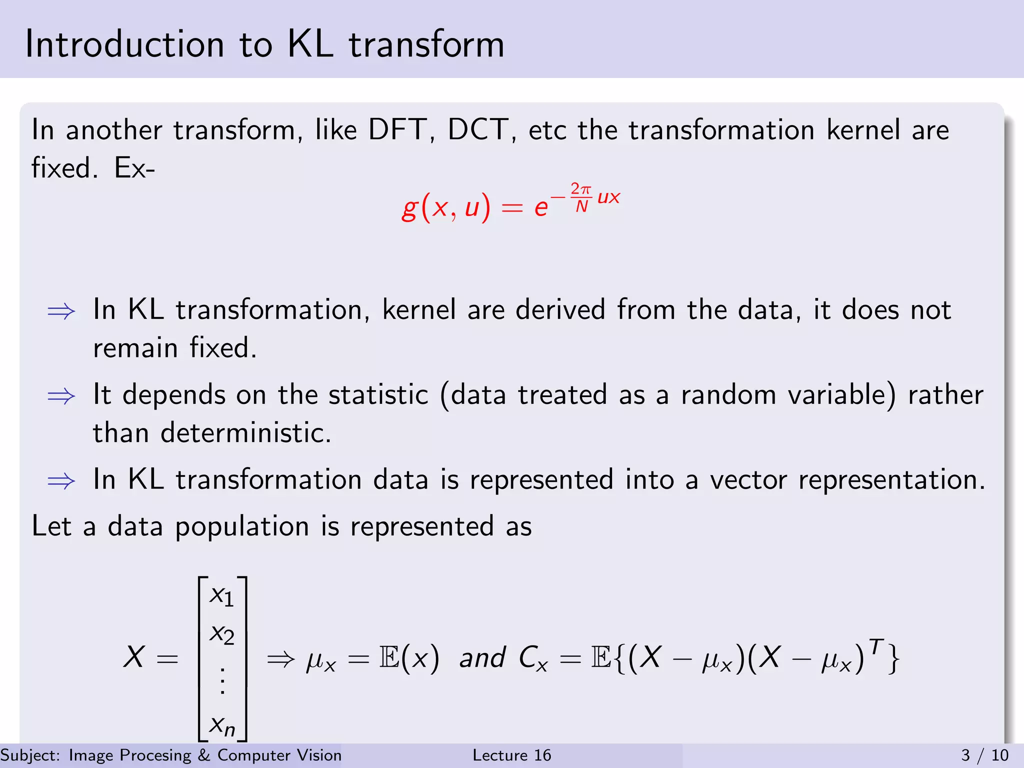
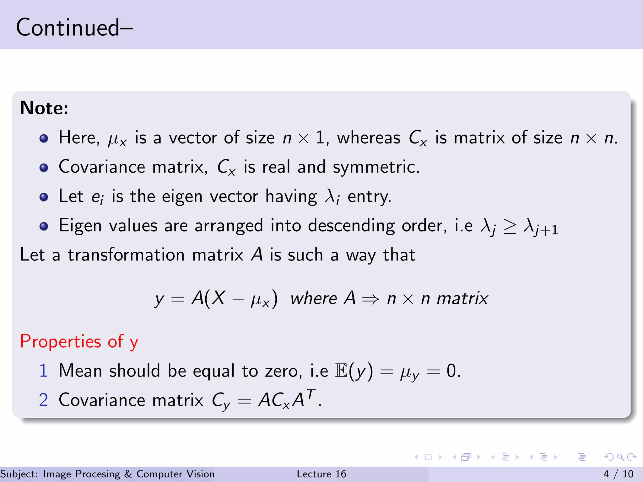
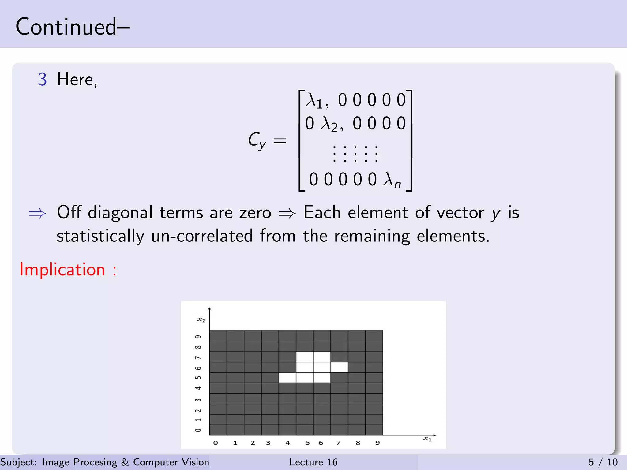
7. Continued–
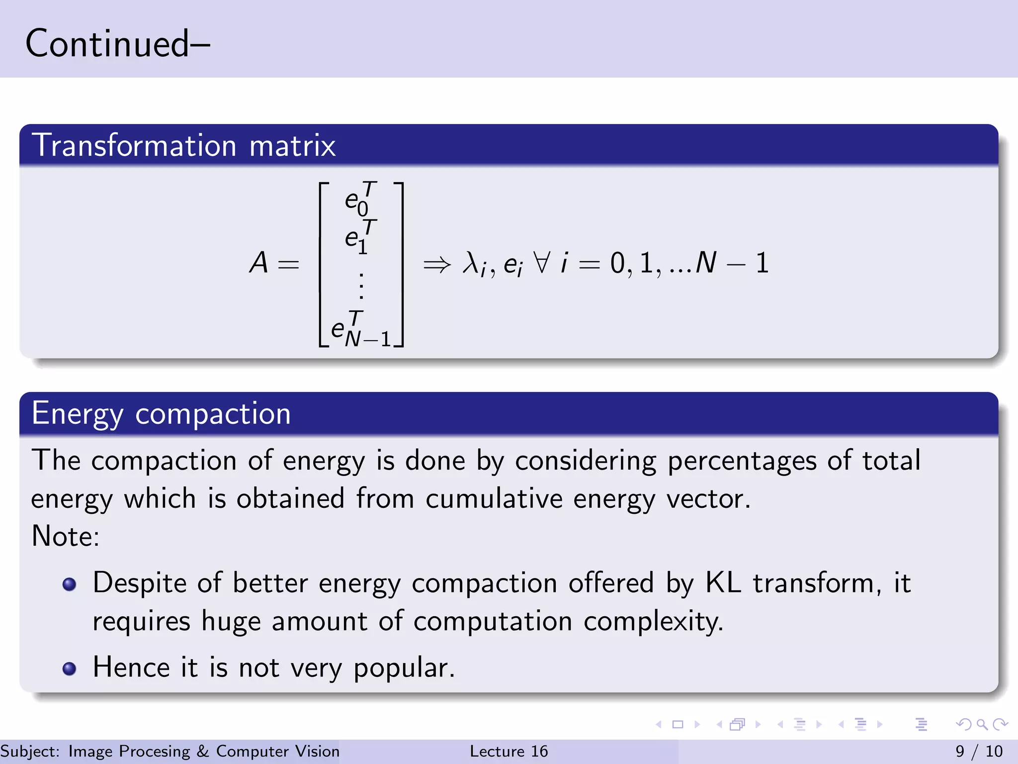
Modified relation
Also, e1 =
0.5696
−0.8219
and e2 =
−0.8219
−0.5696
In this case transformation
matrix A = [e1, e2]. Hence, through KL transformation,
Forwrd transform ⇒ y = A(X − µx ) (5)
Here A−1 = AT . Hence, inverse transform is
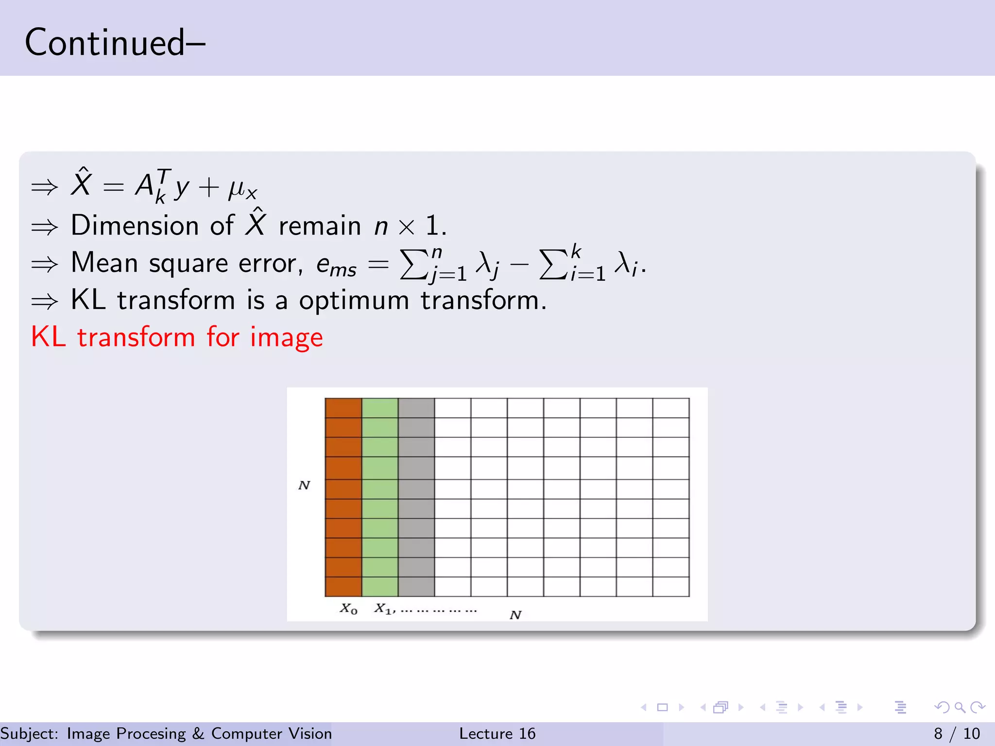
X = AT
y + µx (6)
Let Ak → Matrix having k number of eigen value.
After transformation y = Ak(X − µx ) → Dimension reduces from n × n to
k × n.
Subject: Image Procesing & Computer Vision Dr. Varun Kumar (IIIT Surat)Lecture 16 7 / 10

8. Continued–
⇒ ˆX = AT
k y + µx
⇒ Dimension of ˆX remain n × 1.
⇒ Mean square error, ems = n
j=1 λj − k
i=1 λi .
⇒ KL transform is a optimum transform.
KL transform for image
Subject: Image Procesing & Computer Vision Dr. Varun Kumar (IIIT Surat)Lecture 16 8 / 10

9. Continued–
Transformation matrix
A =





eT
0
eT
1
...
eT
N−1





⇒ λi , ei ∀ i = 0, 1, ...N − 1
Energy compaction
The compaction of energy is done by considering percentages of total
energy which is obtained from cumulative energy vector.
Note:
Despite of better energy compaction offered by KL transform, it
requires huge amount of computation complexity.
Hence it is not very popular.
Subject: Image Procesing & Computer Vision Dr. Varun Kumar (IIIT Surat)Lecture 16 9 / 10

10. References
M. Sonka, V. Hlavac, and R. Boyle, Image processing, analysis, and machine vision.
Cengage Learning, 2014.
D. A. Forsyth and J. Ponce, “A modern approach,” Computer vision: a modern
approach, vol. 17, pp. 21–48, 2003.
L. Shapiro and G. Stockman, “Computer vision prentice hall,” Inc., New Jersey,
2001.
R. C. Gonzalez, R. E. Woods, and S. L. Eddins, Digital image processing using
MATLAB. Pearson Education India, 2004.
Subject: Image Procesing & Computer Vision Dr. Varun Kumar (IIIT Surat)Lecture 16 10 / 10