Downloaded 257 times
![Spatial Domain Methods
• As indicated previously, the term spatial domain refers
to the aggregate of pixels composing an image.
• Spatial domain methods are procedures that operate
directly on these pixels.
• Spatial domain processes will be denoted by the
expression:
g(x,y) = T [f(x,y)]
Where f(x,y) in the input image, g(x,y) is the processed
image and T is as operator on f, defined over some
neighborhood of (x,y)
• In addition, T can operate on a set of input images.](https://image.slidesharecdn.com/dipunit2part1-180930101845/75/Image-enhancement-5-2048.jpg)


![Linear Functions
• Image Negatives (Negative Transformation)
– The negative of an image with gray level in the range [0, L-1],
where L = Largest value in an image, is obtained by using the
negative transformation’s expression:
s = L – 1 – r
Which reverses the intensity levels of an input image, in this
manner produces the equivalent of a photographic negative.
– The negative transformation is suitable for enhancing white
or gray detail embedded in dark regions of an image,
especially when the black area are dominant in size](https://image.slidesharecdn.com/dipunit2part1-180930101845/75/Image-enhancement-15-2048.jpg)


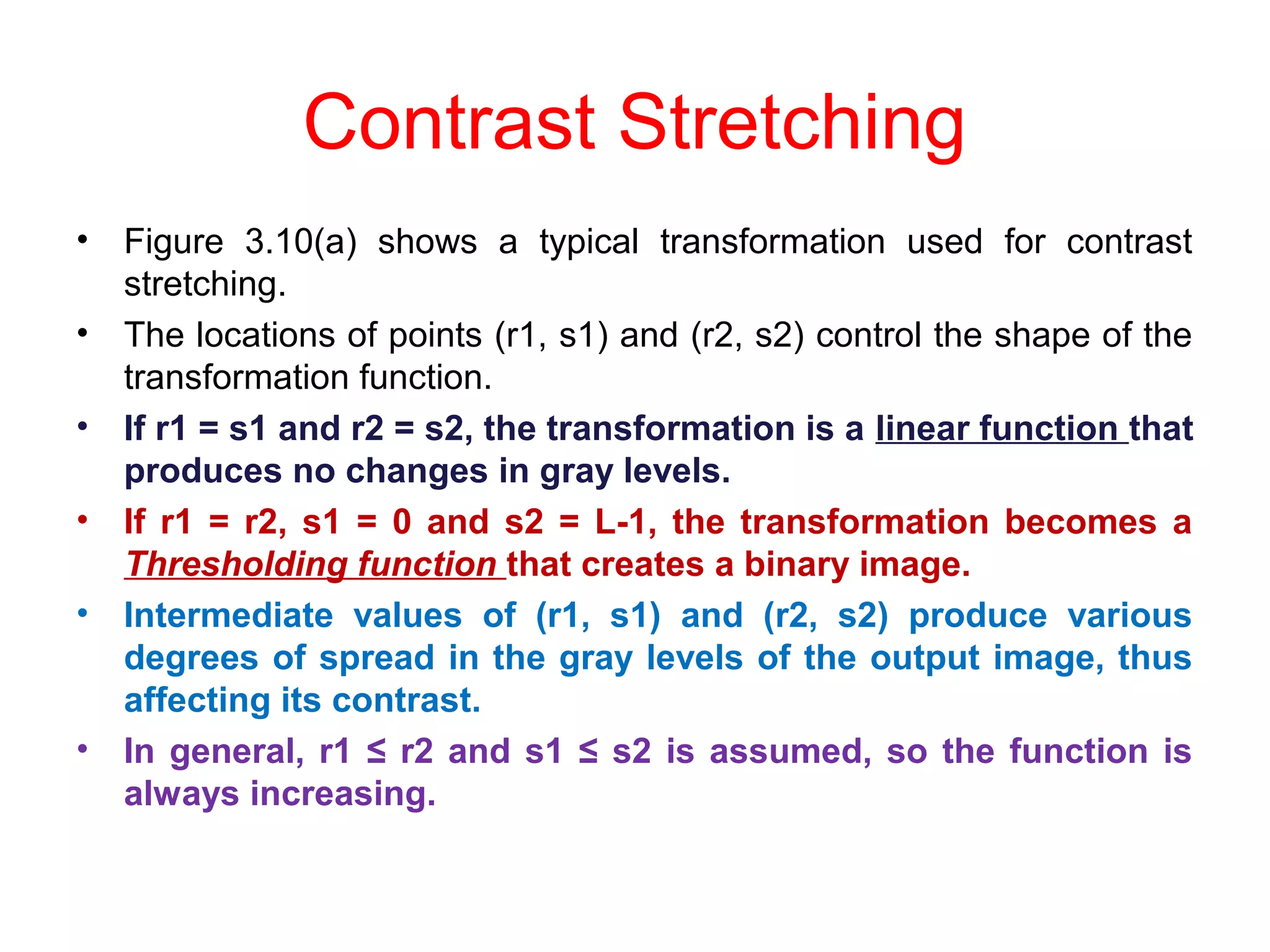
![Contrast Stretching
• Figure 3.10(b) shows an 8-bit image with low contrast.
• Fig. 3.10(c) shows the result of contrast stretching, obtained by
setting (r1, s1) = (rmin, 0) and (r2, s2) = (rmax,L-1) where rmin and rmax
denote the minimum and maximum gray levels in the image,
respectively. Thus, the transformation function stretched the levels
linearly from their original range to the full range [0, L-1].
• Finally, Fig. 3.10(d) shows the result of using the thresholding
function defined previously, with r1=r2=m, the mean gray level in the
image.](https://image.slidesharecdn.com/dipunit2part1-180930101845/75/Image-enhancement-31-2048.jpg)


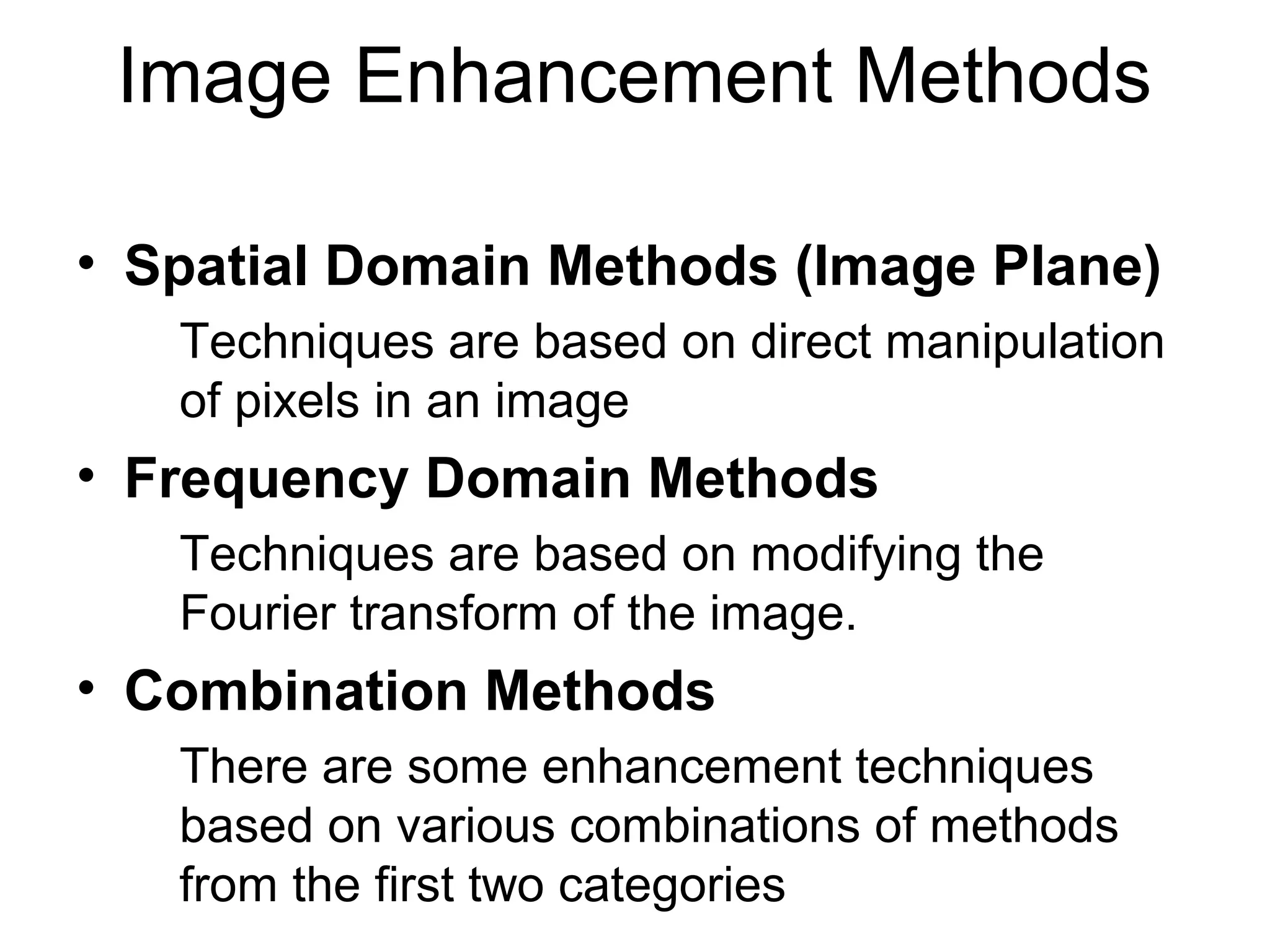
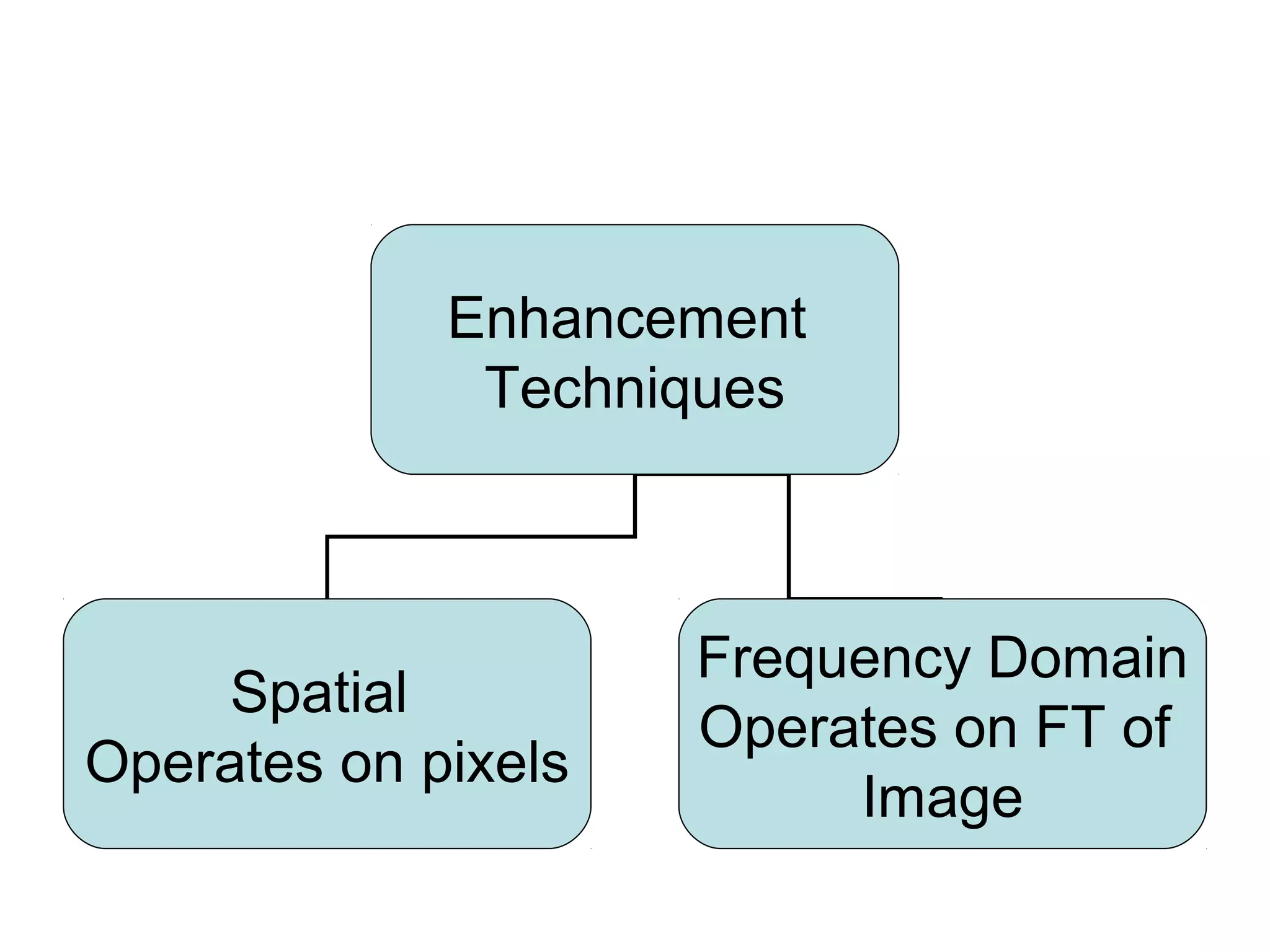
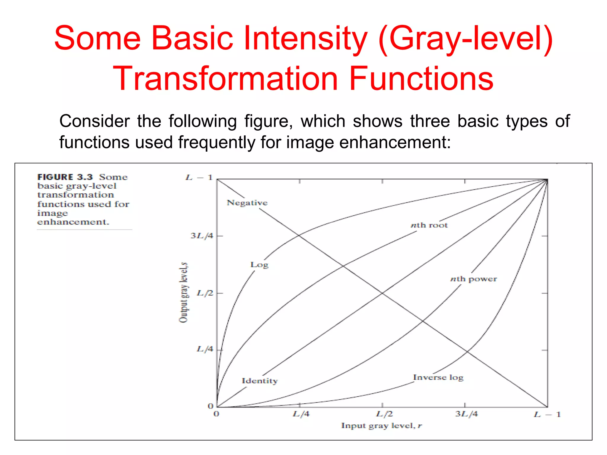
Digital images can be enhanced in various ways to improve quality. There are three main categories of enhancement techniques: spatial domain, frequency domain, and combination methods. Spatial domain methods operate directly on pixel values using point processing or neighborhood filtering. Key spatial techniques include contrast stretching, thresholding, and histogram equalization. Frequency domain methods modify an image's Fourier transform. Common transformations include logarithmic, power-law, and piecewise linear functions, which can increase contrast or highlight certain grayscale ranges. Proper enhancement improves an image's features for desired applications.