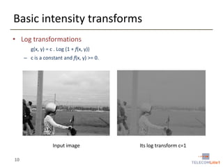
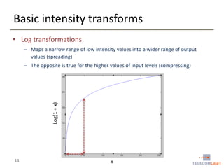
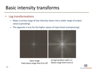
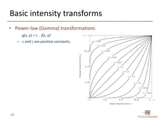
Download as PDF, PPTX

![Histogram equalization
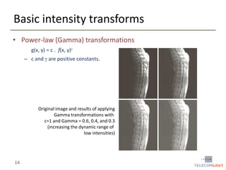
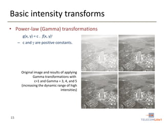
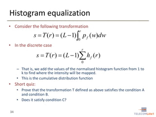
• Goal
• Increase the global contrast of an image by design a transformation (mapping) T
that that makes pixel intensities uniformly distributed over the whole range [0, L-1]
• Input
• An image f of intensity levels in [0, L-1]
• Intensity levels can be viewed as random variables
• Let’s hf be the normalized histogram of f.
hf is also the probability distribution function which we denote by Pf
• We denote by r intensity values of f
• Output
• An image g = T(f) such that the intensities of g are uniformly over the range [0, L1].
• This will improve the contrast by spreading out the most frequent intensity values
• We denote by s = T(r).
30](https://image.slidesharecdn.com/4-131231192701-phpapp02/85/4-intensity-transformations-30-320.jpg)
![Histogram equalization
• We want to compute
• An image g = T(f) such that the intensities of g are better distributed on the
histogram hg
• hg as a PDF, the intensities of g should follow a uniform distribution.
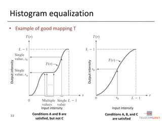
• Requirements for a good mapping T
• Condition A: T is required to be a monotonically increasing function in the
interval [0, L-1]
• That is if x < y T(x) <= T(y)
• Avoids reversing intensities
• Condition B: x [0, L-1] T(x) [0, L-1]
• This guarantees that the range of output intensities are the same as the range of input
intensities.
• Condition C: You may require strict monotonicity
• x < y T(x) < T(y)
• This guarantees the mapping (or transformation )T is one-to-one.
32](https://image.slidesharecdn.com/4-131231192701-phpapp02/85/4-intensity-transformations-32-320.jpg)
![Histogram equalization
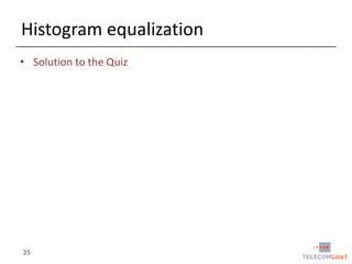
• Interesting property
• If we apply the transformation T to the image f we get an image g of
histogram hg such that
1
s [1, L 1], hg (s)
L 1
• This is a uniform distribution !!!
36](https://image.slidesharecdn.com/4-131231192701-phpapp02/85/4-intensity-transformations-36-320.jpg)
![Histogram equalization – Algorithm
• Input
• A discrete image f of L levels of intensity
• Algorithm
• Step1: Compute the normalized histogram hf of input image f
• Step 2: Compute the CDF of hf, denoted CDFhf
• Step 3: Find a transformation T: [0, L-1] [0, L-1] such that
r
T (r ) ( L 1) h(q ) ( L 1)CDFhf (r )
q 0
• Step 4: Apply the transformation on each pixel of the input image f
• Propert ies
• The procedure is fully automatic and very fast
• Suitable for real-time applications
37](https://image.slidesharecdn.com/4-131231192701-phpapp02/85/4-intensity-transformations-37-320.jpg)
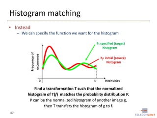
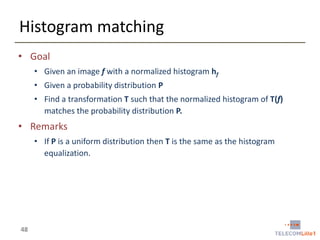
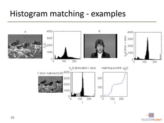
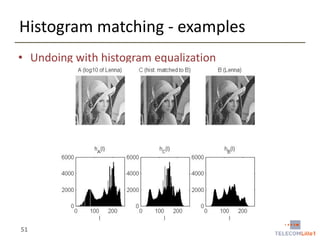
![Histogram matching - procedure
• Input
• A source image f and a target distribution function P
• P can be the normalized histogram of another image g
• Procedure
• Calculate the histogram hf of f
• Calculate the CDFf of f and the CDFP of P
• For each gray level x [0, L-1], find the gray level y for which
• CDFf(x) = CDFP(y)
• We denote this mapping by M
• Can be implemented as a lookup table
• Apply the mapping M to all pixels of the input image f
49](https://image.slidesharecdn.com/4-131231192701-phpapp02/85/4-intensity-transformations-49-320.jpg)

Digital Image Processing covers intensity transformations that can be performed on images. These include basic transformations like negatives, log transformations, and power-law transformations. It also discusses image histograms, which measure the frequency of each intensity level in an image. Histogram equalization aims to improve contrast by mapping intensities to produce a uniform histogram. It works by spreading out the most frequent intensity values.