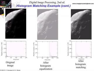
The document discusses the concepts of histogram processing and histogram equalization in digital image processing, outlining methods for enhancing image contrast by transforming pixel value distributions. It introduces key functions and their properties, emphasizing the importance of normalized histograms and transformation functions in achieving uniform pixel distributions. Additionally, it covers histogram matching techniques for transforming images based on predefined probability density functions.

![Digital Image Processing, 2nd ed. www.imageprocessingbook.com
© 2002 R. C. Gonzalez & R. E. Woods
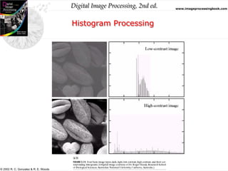
Histogram Processing
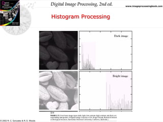
• The histogram of a digital image with intensity levels in the
range [0,L-1] is a discrete function h(rk) = nk, where rk is
the kth intensity value and nk is the number of pixels in the
image with intensity rk.
• A normalized histogram is given by p(rk) = nk/MN for
k=0,1,2,….,L-1.](https://image.slidesharecdn.com/histogramequalizationandmatching-240812102619-ab16b926/85/Histogram-equalization-and-matching-Digital-Image-Processing-8-320.jpg)
![Digital Image Processing, 2nd ed. www.imageprocessingbook.com
© 2002 R. C. Gonzalez & R. E. Woods
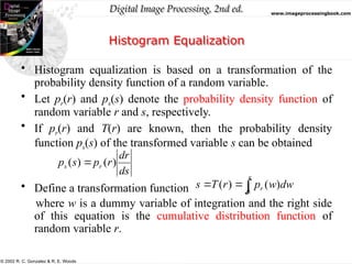
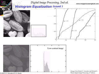
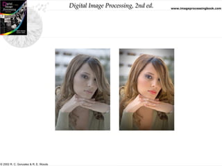
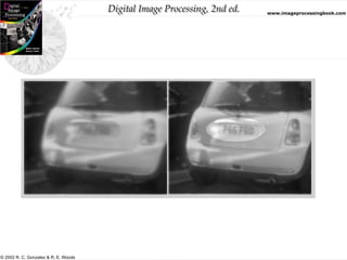
Histogram Equalization
• Histogram equalization:
– To improve the contrast of an image
– To transform an image in such a way that the transformed image has a
nearly uniform distribution of pixel values
• Transformation:
– Assume r has been normalized to the interval [0,1], with r = 0
representing black and r = 1 representing white
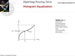
– The transformation function satisfies the following conditions:
• T(r) is single-valued and monotonically increasing in the interval
•
1
0
r
1
0
for
1
)
(
0
r
r
T
1
0
)
(
r
r
T
s](https://image.slidesharecdn.com/histogramequalizationandmatching-240812102619-ab16b926/85/Histogram-equalization-and-matching-Digital-Image-Processing-11-320.jpg)