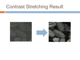
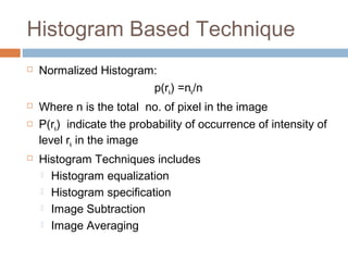
This document summarizes techniques for image enhancement in both the spatial and frequency domains. In the spatial domain, point processing techniques like contrast stretching can modify pixel intensities, while histogram equalization spreads out the most frequent intensities. Mask processing techniques apply operators to local neighborhoods. Frequency domain techniques modify image Fourier coefficients and take the inverse transform to obtain the enhanced image. Common operations include noise filtering and sharpening.

1. CHAPTER6
IMAGE ENHANCEMENT
Dr. Varun Kumar Ojha
and
Prof. (Dr.) Paramartha Dutta
Visva Bharati University
Santiniketan, West Bengal, India

2. Image Enhancement
 Necessity of Image Enhancement
 Spatial Domain Operation
 Frequency Domain Operation
Back to Course Content Page
Click Here

3. Image Enhancement
 Image Enhancement: It is processing of
enhancement of certain feature of image
 Removal of noise
 Increasing contrast for a dark image etc.
 Choice of image enhancement technique are vary
from problem to problem
 i.e. Best technique fro enhancement of X-Ray
image may not be suitable for enhancement of
microscopic images.

4. Image Enhancement
 There are two image enhancement technique
 Spatial Domain Technique
 Work on image plane itself
 Discrete manipulation of pixels in an image
 Frequency Domain Technique
 Modify Fourier Transform coefficient of image and
taking inverse Fourier Transform of modified image to
obtain modified image

5. Back to the chapter content
Click Here

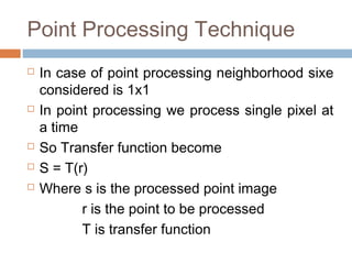
6. Spatial Domain Operation
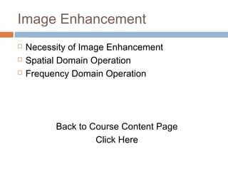
 Let we image f(x,y) then
g(x,y) = T[f(x,y)]
 Where T [ . ] is the transfer function which
transform the input image f(x,y) (which need to
be enhanced) to enhanced image g(x,y)
 The operator T operates at point (x,y)
considering certain neighborhood of the point
(x,y) of the image
 Similarly for a single pixel x we can write
g(x) = T[f(x)]

7. Spatial Domain Operation
p
y
x
Input Image f(x,y)
3 x 3 neighborhood at
point (x,y)
For different technique neighborhood
size may be different depending
upon the type of image and type of
operation

8. Spatial Domain Operation
 Spatial domain operation includes
 Point Processing Techniques
 Histogram Based Technique
 Mask Processing Technique

9. Point Processing Technique
 In case of point processing neighborhood sixe
considered is 1x1
 In point processing we process single pixel at
a time
 So Transfer function become
 S = T(r)
 Where s is the processed point image
r is the point to be processed
T is transfer function

10. Point Processing Technique
s
lightDark
light
r
T(r)
Dark
s
lightDark
light
r
T(r)
Dark
Type of Transfer function
Narrow range in
original image
Wider range
in processed
image
Thresholding Transfer
function

11. Point Processing Technique
 Point Processing Technique Includes
 Image Negative
 Contrast Stretching
 Gray Level Slicing

12. Image Negative
 Light image converted to darker image
 Darker image converted to lighter image
s
L -1
s = T(r) = L-1-r
r
L -1
This kind of Transfer function is very useful in medical science
0
Concept:
max intensity → min intensity
min intensity → max intensity

13. Image Negative Result
Cancer region detection

14. Contrast Stretching
 Contrast image is process of increasing low
contrast image to high contrast image
s
L -1
s = T(r)
r
L -1
0
Concept:
Narrow intensity range in original
image is converted wide intensity
range in processed image
For enhancement operation
r1 ≤ r2 and s1 ≤ s2
For r1 = r2 , s1 = 0 and s2 = L-1 the
transfer function become thresholding
operation
(r1,s1)
(r2,s2)

15. Contrast Stretching Result

16. Gray Level Slicing
s
L -1
r
L -1
0
A B
s
L -1
r
L -1
0
A B
Concept:
Here it shows that only in the
range A – B the image is
enhanced and for all other pixel
value are suppressed
Concept:
Here it shows that only in the
range A – B the image is
enhanced and all other pixel
value are retained

17. Gray Level Slicing Results

18. Histogram Based Technique
 Histogram Definition
 A image having (0 , L-1) discrete intensity
level
 Then Histogram:
h(rk) = nk
 Where rk: Intensity level
 nk: No. of pixel having intensity level rk
 The plot of distinct intensity level against all
possible intensity level is known at Histogram

19. Histogram Based Technique
 Normalized Histogram:
p(rk) =nk/n
 Where n is the total no. of pixel in the image
 P(rk) indicate the probability of occurrence of intensity of
level rk in the image
 Histogram Techniques includes
 Histogram equalization
 Histogram specification
 Image Subtraction
 Image Averaging

20. Histogram Based Technique

21. Histogram Based Technique

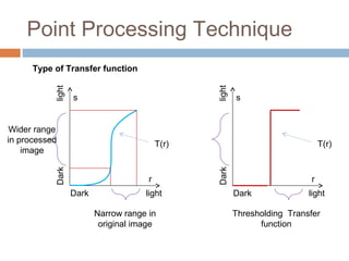
22. Histogram Equalization
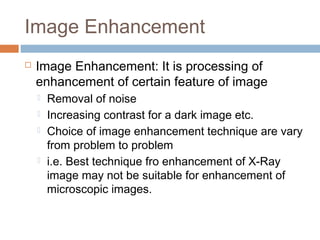
 Let r represents gray level in an image
 Assume [0,1] is the normalized pixel in the image where 0 →
back pixel and 1 → white pixel
s = T(r)
 where r is the intensity in original image and s is the intensity
in the processed image
 We assume the transfer function satisfy the following
condition
1. T(r) must be a single valued & monotonically increasing
in the range 0 ≤ r ≤ 1 i.e. Darker pixel remains darker in
the processed image
2. 0 ≤ T(r) ≤ 1 for 0 ≤ r ≤ 1 i.e. any pixel intensity vale may
not be larger than the maxim intensity level.

23. Histogram Equalization
 Inverse Transfer
r = T-1
(s)
 It should also satisfy the above condition
 For continuous domain
 pr(r) → pdf of r
 ps(s) → pdf of s
 For elementary probability theory we know that if pr(r)
and ps(s) are known and T-1(s) is single valued
monotonically increasing function
 Then we can obtained
ps(s) = pr(r)|dr/ds|at r = T-1(s)

24. Histogram Equalization
 Now we take transfer function
 s = T(r) = ∫0→ r pr(w) dw
 From this we can compute
ds/dr = pr(r)
 ps(s) = pr(r) |dr/ds|
 = pr(r). 1/pr(r) = 1
 Discrete Formulation
 pr(rk) = nk/n
 Histogram equalization become
sk = T(rk) = ∑i= 0 – k pr(ri)
= ∑i= 0 – k ni/n

25. Histogram Equalization

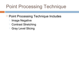
26. Histogram
Specification/Matching
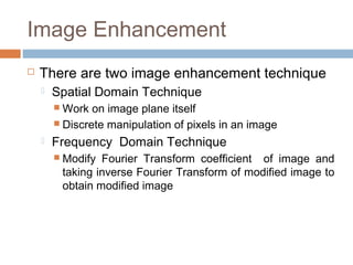
 Target Histogram
 Let r → given image and z → target area in the image
 Hence pz(z) → target histogram
 s = T(r) = ∫0→ r pr(w) dw
 Similarly we have function G(z) instead T(r) for target
histogram
 G(z) = ∫0→ z pz(t) dt
 Discrete formulation
sk = T(rk) =∑i= 0 – k ni/n
Let pz(z) is the specified target histogram
Vk = G(zk) = ∑i= 0 – k pz(zi) = sk
Zk =G-1
[T(rk)]

27. Histogram
Specification/Matching
Graphical interpretation
of mapping from rk to sk
via T(r).
Mapping of zq to its
corresponding value
vq via G(z).
Inverse mapping from sk
to its corresponding
value of zk

28. Example Histogram
 Preparing..

29. Image Differencing
g(x,y) = f(x,y) – h(x,y)
 where h(x,y) is the image subtracted from image f(x,y)
 Application of Image Subtraction
 Mask mode radiography: ( It is a image differencing
preprocess for showing oriental diseases.)
 In this case h(x, y), the m ask, is an X-ray im ag e o f a re g io n o f a
patie nt’s bo dy capture d by an intensified TV camera (instead of
traditional X-ray film) located opposite an X-ray source. The
procedure consists of injecting a contrast medium into the patient’s
bloodstream, taking a series of images of the same anatomical
region as h(x, y), and subtracting this mask from the series of
incoming images after injection of the contrast medium. The net
effect of subtracting the mask from each sample in the incoming
stream of TV images is that the areas that are different between f(x,
y) and h(x, y) appear in the output image as enhanced detail.

30. Application Image Differencing
Mask image.
An image (taken after
injection of a contrast
medium into the
bloodstream) with mask
subtracted out

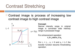
31. Image Averaging
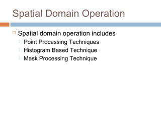
g(x,y) = f(x,y) + η(x,y)
g’(x,y) = 1/k ∑i = 1 to K gi(x,y)
E [g’(x,y) ] = f(x,y)
 Application in Astronomical Field
 Noise reduction by image averaging
average of k frames
Error (noise must be zero mean)

32. Image Averaging Result
a b c
fed
(a) Image of Galaxy Pair NGC 3314. (b) Image corrupted by additive Gaussian
noise with zero mean and a standard deviation of 64 gray levels. (c)–(f) Results
of averaging K=8, 16, 64, and 128 noisy images.

33. Mask Processing Techniques
 Preparing..

34. Back to the chapter content
Click Here

35. Frequency Domain Operation
 Preparing…

36. Back to the chapter content
Click Here