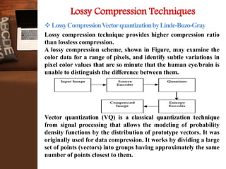
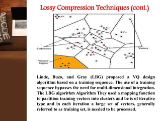
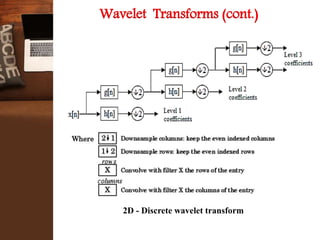
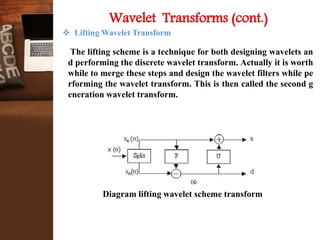
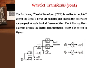
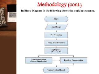
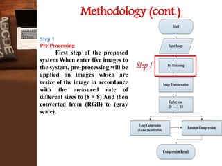
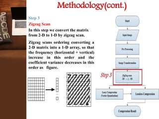
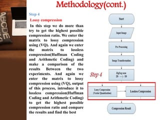
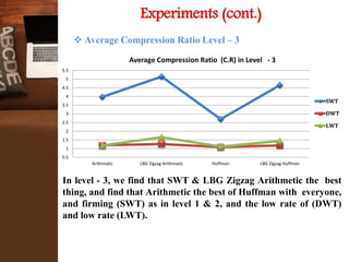
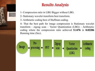
This document provides an overview of a research project on image compression. It discusses image compression techniques including lossy and lossless compression. It describes using discrete wavelet transform, lifting wavelet transform, and stationary wavelet transform for image transformation. Experiments were conducted to compare the compression ratio and processing time of different combinations of wavelet transforms, vector quantization, and Huffman/Arithmetic coding. The results were analyzed to evaluate the compression performance and efficiency of the different methods.

2. Produced by
Omar Ghazi Abbood Khukre
Master Student in Department of Information
Technology, Institute of Graduate Studies and Research,
Alexandria University, Egypt
.

3. Contents
Introduction
Image Compression Definition
Image Compression Types
Wavelet Transforms
Problem Statement
Objective
Methodology
Experiments and Results Analysis
Conclusion
Future work

4. INTRODUCTION
 Image Compression: It is the Art & Science of reducing the amount of
data required to represent an image.
 It is the most useful and commercially successful technologies in the
field of Digital Image Processing.
 The number of images compressed and decompressed daily is
innumerable.
 Web page images & High-resolution digital camera photos also are also
compressed to save storage space & reduce transmission time.
 The researchers have faced in the field of Image compression some
difficulties especially in get the best accuracy of the image with a high
compression ratio.
 This research aims an improving the image compression process to the
maximum extent.

5. Image Compression Definition
Image compression is minimizing the size in bytes
of a graphics file without degrading the quality of
the image to an unacceptable level .
The reduction in file size allows more images
to be stored in a given amount of disk or memory
space. It also reduces the time required for
images to be sent over the Internet or downloaded
from Web pages.

6.  Lossy Compression Techniques
In information technology, lossy compression or irreversible
compression is the class of data encoding methods that uses
inexact approximations and partial data discarding to represent
the content. These techniques are used to reduce data size for
storage, handling, and transmitting content. The amount of data
reduction possible using lossy compression is often much higher
than through lossless techniques.
 Lossless Compression Techniques
Lossless compression is a class of data compression
algorithms that allows the original data to be perfectly
reconstructed from the compressed data. By contrast, lossy
compression permits reconstruction only of an approximation of
the original data, though this usually improves compression rates
(and therefore reduces file sizes)
Image Compression Types

7. Lossy Compression Techniques
LossyCompressionVectorquantizationbyLinde-Buzo-Gray
Lossy compression technique provides higher compression ratio
than lossless compression.
A lossy compression scheme, shown in Figure, may examine the
color data for a range of pixels, and identify subtle variations in
pixel color values that are so minute that the human eye/brain is
unable to distinguish the difference between them.
Vector quantization (VQ) is a classical quantization technique
from signal processing that allows the modeling of probability
density functions by the distribution of prototype vectors. It was
originally used for data compression. It works by dividing a large
set of points (vectors) into groups having approximately the same
number of points closest to them.

8. Linde, Buzo, and Gray (LBG) proposed a VQ design
algorithm based on a training sequence. The use of a training
sequence bypasses the need for multi-dimensional integration.
The LBG algorithm Algorithm They used a mapping function
to partition training vectors into clusters and be is of iterative
type and in each iteration a large set of vectors, generally
referred to as training set, is needed to be processed.
Lossy Compression Techniques (cont.)

9. Wavelet Transforms
Represent an image as a sum of wavelet functions (wavelets)
with different locations and scales. Any decomposition of an
image into wavelets involves a pair of waveforms: one to
represent the high frequencies corresponding to the detailed
parts of an image and one for the low frequencies or smooth
parts of an image.

10.  Discrete Wavelet Transform
The Discrete Wavelet Transform (DWT) of image signals produces
a nonredundant image representation, which provides better
spatial and spectral localization of image formation, compared
with other multi scale representations such as Gaussian and
Laplacian pyramid. Recently, Discrete Wavelet Transform has
attracted more and more interest in image fusion .An image can
be decomposed into a sequence of different spatial resolution
images using DWT.In case of a 2D image, an N level decomposition
can be performed resulting in 3N+1 different frequency bands and
it is shown in figure.
Wavelet Transforms (cont.)

11. Wavelet Transforms (cont.)
2D - Discrete wavelet transform

12.  Lifting Wavelet Transform
The lifting scheme is a technique for both designing wavelets an
d performing the discrete wavelet transform. Actually it is worth
while to merge these steps and design the wavelet filters while pe
rforming the wavelet transform. This is then called the second g
eneration wavelet transform.
Wavelet Transforms (cont.)
Diagram lifting wavelet scheme transform

13.  Stationary Wavelet Transform
The stationary wavelet transform (SWT) is a wavelet transform
algorithm designed to overcome the lack of translation invariance
of the Discrete Wavelet Transform (DWT). Translation invariance
is achieved by removing the down samplers and up samplers in
the Discrete Wavelet Transform (DWT) and up sampling the filter
coefficients by a factor of in the level of the algorithm. The SWT
is an inherently redundant scheme as the output of each level of
SWT contains the same number of samples as the input.
Wavelet Transforms (cont.)

14. The Stationary Wavelet Transform (SWT) is similar to the DWT
except the signal is never sub-sampled and instead the filters are
up sampled at each level of decomposition. The following block
diagram depicts the digital implementation of SWT as shown in
figure.
Wavelet Transforms (cont.)

15. Problem Statement
• The large increase in the data lead to delays in access to the
information required and this leads to a delay in the time. Large
data lead to data units and storage is full this leads to the need
to buy a bigger space for storage and losing money. Large data
lead to give inaccurate results for the similarity of data and this
leads to getting inaccurate information.
• Also to show the difference between the types of transforms
Stationary Wavelet Transform, Discrete Wavelet Transform,
and Lifting Wavelet Transform because they are very similar
at one level so we used three levels.

16. Research Objective
In lossy compression, the compression ratio is
unaccepted. The proposed system suggests an image
compression method of lossy image compression
through the three types of transformations such as
stationary wavelet transform, discrete wavelet
transform , and lifting wavelet transform and the
comparison between the three types and the use of
vector quantization (VQ) to improve the image
compression process.

17. Methodology
The proposed lossy compression approach applied SWT
and VQ techniques in order to compressed input images
in four phases; namely preprocessing, image
transformation, zigzag scan, and lossy/lossless
compression. In figure shows the main steps of the
system that follows the schema independent and image
compression techniques. We discuss how a matrix
arrangement gives us the best compression ratio and
lessloss of the characteristics of the image through
a wavelet transform with lossy compression techniques.

18. Methodology (cont.)
In Block Diagram in the following shows the work in sequence.

19. Methodology (cont.)
Step 1
Pre Processing
First step of the proposed
system When enter five images to
the system, pre-processing will be
applied on images which are
resize of the image in accordance
with the measured rate of
different sizes to (8 × 8) And then
converted from (RGB) to (gray
scale).

20. Methodology(cont.)
Step 2
Wavelet transforms
Image transformation phase
received the resizable gray
scale images and produced
transformed images. This
phase used the three types of
wavelet transforms such as
DWT, LWT, and SWT.

21. Methodology(cont.)
Step 3
Zigzag Scan
In this step we convert the matrix
from 2-D to 1-D by zigzag scan.
Zigzag scans ordering converting a
2-D matrix into a 1-D array, so that
the frequency (horizontal + vertical)
increase in this order and the
coefficient variance decreases in this
order as figure.

22. Step 4
Lossy compression
In this step we do more than
try to get the highest possible
compression ratio. We enter the
matrix to lossy compression
using (VQ). And again we enter
the matrix to lossless
compression(Huffman Coding
and Arithmetic Coding) and
make a comparison of the
results Between the two
experiments. And again we
enter the matrix to lossy
compression using (VQ), output
of this process, introduce it to
lossless compression(Huffman
Coding and Arithmetic Coding)
to get the highest possible
compression ratio and compare
the results and find the best
Methodology(cont.)

23. Methodology(cont.)
Compression Ratio
Compression Ratio: is the ratio of size of the compressed database
system with the original size of the uncompressed database
systems. Also known as compression power is a computer-science
term used to quantify the reduction in data-representation size
produced by a data compression algorithm. Compression ratio is
defined as follows:
Compression Time
• Compression Time = represents the elapsed time during the
compression process.

24. Experiments and Results Analysis
Experiments
In this section of the performance of three types of wavelet transform
(SWT, DWT, and LWT) and the impact of each type on the image
lossy compression performance also it shows the lossy using vector
quantization (LBG) and lossless compression using Arithmetic coding
and Huffman coding.
The First Experiment
In this experiment, four operations:
 1- DWT-Zigzag-Arithmetic
 2- DWT-Zigzag-LBG–Arithmetic
 3- DWT-Zigzag-Huffman
 4- DWT-Zigzag-LBG–Huffman
Table 1 showing results for the process lossy and lossless image
compression to the five images using the discrete wavelet transform
with arithmetic coding and huffman coding without the use of the
LBG, as well as with the use of the LBG and that using three
decomposition levels.

25. Experiments (cont.)
Discrete wavelet transform, vector quantization (LBG), Arithmetic and Huffman coding
DWT
DWT Zigzag
Arithmetic
DWT Zigzag LBG &
Arithmetic
DWT Zigzag
Huffman
DWT Zigzag LBG &
Huffman
Image Level C.Ratio
Running
time(Sec) C.Ratio psnr
Running
time(Sec) C.Ratio
Running
time(Sec) C.Ratio psnr
Running
time (Sec)
Lena
1 1.1934 0.4919 1.2549 18.2975 0.0157 1.1403 0.0735 1.1879 18.2975 0.057
2 1.261 0.0459 1.3027 18.2745 0.012 1.0556 0.0785 1.1403 18.2745 0.0438
3 1.2994 0.0721 1.28 18.2449 0.0164 1.026 0.1237 1.1583 18.2449 0.0465
Camera
man
1 1.2518 0.0351 1.2549 18.2588 0.0158 1.177 0.0611 1.2549 18.2588 0.0421
2 1.2549 0.0498 1.2641 18.1648 0.0125 1.1557 0.0904 1.2047 18.1648 0.0459
3 1.2896 0.062 1.2457 18.0733 0.0111 1.1454 0.1148 1.2018 18.0733 0.0609
Tulips
1 1.1851 0.093 1.2427 17.4091 0.0153 1.1824 0.1483 1.199 17.4091 0.0657
2 1.1934 0.0965 1.28 17.4196 0.0105 1.177 0.1231 1.199 17.4196 0.0458
3 1.0916 0.1131 1.2864 17.3919 0.011 1.1479 0.2548 1.1824 17.3919 0.0447
White
flower
1 1.0622 0.0431 1.2549 16.7503 0.0128 1.0385 0.0764 1.1879 16.7503 0.0413
2 1.1203 0.0546 1.2549 16.7639 0.0106 1.0893 0.075 1.1934 16.7639 0.0458
3 1.0916 0.0457 1.2518 16.8377 0.0169 1.026 0.0785 1.1879 16.8377 0.047
Fruits
1 1.2047 0.0489 1.28 17.5693 0.013 1.1428 0.0829 1.2104 17.5693 0.0513
2 1.2104 0.0922 1.2427 17.6137 0.0139 1.1302 0.0967 1.2161 17.6137 0.044
3 1.2161 0.0508 1.2641 17.5718 0.0148 1.1252 0.0831 1.1962 17.5718 0.0455

26. Experiments (cont.)
The Second Experiment
In this experiment, four operations:
 1- LWT-Zigzag-Arithmetic
 2- LWT-Zigzag-LBG–Arithmetic
 3- LWT-Zigzag- Huffman
 4- LWT-Zigzag-LBG–Huffman
Table 2 showing results for the process lossy and lossless
image compression to the five images using the lifting
wavelet transform with arithmetic coding and huffman
coding without the use of the LBG, as well as with the
use of the LBG and that using three decomposition levels
.

27. Experiments (cont.)
Lifting wavelet transform, vector quantization (LBG), Arithmetic and Huffman coding
LWT
LWT Zigzag
Arithmetic
LWT Zigzag LBG &
Arithmetic
LWT Zigzag
Huffman
LWT Zigzag LBG &
Huffman
Image Level C.Ratio
Running
time (Sec)
C.Ratio psnr
Running
time (Sec)
C.Ratio
Running
time (Sec)
C.Ratio psnr
Running
time (Sec)
Lena
1 1.4065 0.3177 1.6842 13.1876 0.0081 1.3763 0.0674 1.4545 13.1876 0.0216
2 1.3763 0.4231 1.641 11.9784 0.0097 1.113 0.0527 1.4712 11.9784 0.0162
3 1.1636 0.0489 1.6842 17.4394 0.0073 1.094 0.0708 1.4545 17.4394 0.0154
Camera
man
1 1.5421 0.0658 1.641 13.6895 0.0076 1.2673 0.0511 1.4712 13.6895 0.017
2 1.2427 0.0326 1.7534 12.7065 0.0093 1.1327 0.0401 1.4222 12.7065 0.0155
3 1.1428 0.0376 1.6623 16.9649 0.0074 1.1228 0.0836 1.4222 16.9649 0.0204
Tulips
1 1.0275 0.0947 1.7777 16.2979 0.0122 1.3763 0.1357 1.4545 17.0032 0.0196
2 1.4382 0.1336 1.641 12.2671 0.0111 1.094 0.1054 1.4712 12.2671 0.0225
3 1.2549 0.1174 1.6842 19.5465 0.0073 1.0578 0.1067 1.4545 19.5465 0.0162
White
flower
1 1.3913 0.04 1.641 15.4661 0.0073 1.3763 0.0537 1.4712 15.4661 0.0182
2 1.3061 0.0473 1.7066 14.3703 0.0118 1.2549 0.0528 1.4545 14.3703 0.0186
3 1.1636 0.0827 1.641 16.1241 0.0074 1.2549 0.0599 1.4712 16.1241 0.0162
Fruits
1 1.2397 0.0453 1.7777 12.3394 0.0091 1.1228 0.0557 1.4065 12.3394 0.016
2 1.3763 0.079 1.641 12.2289 0.0089 1.113 0.0902 1.4712 12.2289 0.0164
3 1.1962 0.0874 1.6202 18.1602 0.0074 1.0756 0.0652 1.4065 18.1602 0.0164

28. Experiments (cont.)
The Third Experiment
In this experiment, four operations:
 1- SWT-Zigzag-Arithmetic
 2- SWT–Zigzag-LBG–Arithmetic
 3- SWT-Zigzag- Huffman
 4- SWT–Zigzag-LBG–Huffman
In the table 3, showing results for the process lossy and lossless
image compression to five images using stationary wavelet
transform with arithmetic coding and Huffman coding without the
use of the LBG, as well as with the use of the LBG and that using
three decomposition levels.

29. Experiments (cont.)
Stationary wavelet transform, vector quantization (LBG), Arithmetic and Huffman coding
SWT
SWT Zigzag
Arithmetic
SWT Zigzag LBG &
Arithmetic
SWT Zigzag
Huffman
SWT Zigzag LBG &
Huffman
Image Level C.Ratio
Running
time(Sec)
C.Ratio psnr
Running
time(Sec)
C.Ratio
Running
time(Sec)
C.Ratio psnr
Running
time(Sec)
Lena
1 4.3667 0.1155 5.0073 18.0121 0.0685 2.6256 0.859 4.8188 18.0121 0.0473
2 4.3667 0.0414 5.0073 18.8982 0.012 2.6256 0.8439 4.8188 18.8982 0.0455
3 4.3667 0.1906 5.0073 18.8982 0.0137 2.6256 0.8576 4.8188 18.8982 0.0422
Camera
man
1 4.1042 0.0651 5.0073 16.8483 0.011 2.6771 0.9157 4.853 16.8483 0.0419
2 4.1042 0.0537 5.0073 18.1099 0.011 2.6771 0.8346 4.853 18.1099 0.0447
3 4.1042 0.0398 5.0073 18.1099 0.0103 2.6771 0.9481 4.853 18.1099 0.0462
Tulips
1 3.8641 0.0934 5.6574 18.6787 0.0099 2.7563 0.8965 4.6022 18.6787 0.0461
2 3.8641 0.0961 5.6574 17.1798 0.0116 2.7563 0.9289 4.6022 17.1798 0.0456
3 3.8641 0.0969 5.6574 17.1798 0.0121 2.7563 0.8919 4.6022 17.1798 0.0421
White
flower
1 3.7372 0.0393 4.9588 17.3002 0.0117 2.7018 0.8483 4.6757 17.3002 0.0459
2 3.7372 0.0392 4.9588 17.2142 0.0128 2.7018 0.8438 4.6757 17.2142 0.0459
3 3.7372 0.041 4.9588 17.2142 0.012 2.7018 0.8411 4.6757 17.2142 0.0412
Fruits
1 3.828 0.0584 5.1072 18.9503 0.0132 2.7379 0.8438 4.3206 18.9503 0.0435
2 3.828 0.458 5.1072 18.1739 0.0105 2.7379 0.8585 4.3206 18.1739 0.0567
3 3.828 0.1188 5.1072 18.1739 0.012 2.7379 0.8463 4.3206 18.1739 0.043

30. Experiments (cont.)
 Average Compression Ratio Level – 1
0.5
1
1.5
2
2.5
3
3.5
4
4.5
5
5.5
Arithmatic LBG Zigzag Arithmatic Huffman LBG Zigzag Huffman
Average Compression Ratio (C.R) in Level -1
SWT
DWT
LWT
In level - 1, we find that SWT & LBG Zigzag arithmetic the best
thing, and find that arithmetic the best of huffman with everyone.

31. Experiments (cont.)
0.5
1
1.5
2
2.5
3
3.5
4
4.5
5
5.5
Arithmatic LBG Zigzag Arithmatic Huffman LBG Zigzag Huffman
Average Compression Ratio (C.R) in Level - 2
SWT
DWT
LWT
 Average Compression Ratio Level – 2
In level - 2 , We find that SWT & LBG Zigzag Arithmetic the best
thing , and find that Arithmetic the best of Huffman with everyone,
and firming (SWT) as in level 1, and the high rate of (DWT) and
low rate (LWT) .

32. Experiments (cont.)
 Average Compression Ratio Level – 3
0.5
1
1.5
2
2.5
3
3.5
4
4.5
5
5.5
Arithmatic LBG Zigzag Arithmatic Huffman LBG Zigzag Huffman
Average Compression Ratio (C.R) in Level - 3
SWT
DWT
LWT
In level - 3, we find that SWT & LBG Zigzag Arithmetic the best
thing, and find that Arithmetic the best of Huffman with everyone,
and firming (SWT) as in level 1 & 2, and the low rate of (DWT)
and low rate (LWT).

33. 1- Compression ratio in LBG Bigger without LBG.
2- Stationary wavelet transform best transform.
3- Arithmetic coding best of Huffman coding.
4- That the best path for image compression is Stationary wavelet
transform - zigzag scan – Vector Quantization (LBG) - Arithmetic
coding where the compression ratio achieved 5.1476 in 0.02286
Running time (Sec).
Results Analysis

34.  This thesis introduced a novel approach that is built to work on
image compression. Our approach used vector quantization LB
G, Arithmetic coding and Huffman coding with three types of wa
velet transforms such as Discrete Wavelet Transform DWT, Lifti
ng Wavelet Transform LWT, and Stationary Wavelet Transform
SWT on three decomposition levels. As in Stationary Wavelet Tr
ansform (SWT) compression ratio is fixed at a high level, and Di
screte Wavelet Transform (DWT) compression ratio variable at a
high level, either Lifting Wavelet Transform (LWT) is less than t
he compression at high level.
 We conclude that arithmetic coding is better than Huffman codi
ng in terms of compression ratio and time. We found that the bes
t way to compression in this system is the stationary wavelet tran
sforms (SWT), LBG vector quantization, and arithmetic coding
where it gives the best compression ratio with less time possible.
Also the size of compressed data by adding arithmetic coding is b
etter than adding Huffman coding to SWT.
CONCLUSION