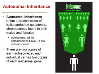
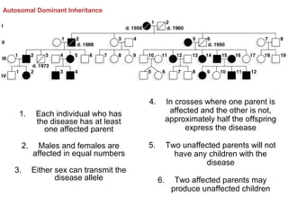
Homework 1 Results!

• You all nailed it! 
• Introduction: 3 pts possible, class average: 2.9
• Chapter 1: 10 pts possible, class average 8.9
• We had a few scores above 10!
• 2% bonus for not opening a hint
Mastering Genetics QUIZ
• Quiz 1: 30 minute time limit, 10 questions! 
– Quiz 2: Coming soon! Same thing!
– Quiz 1 & 2: 10 questions, quiz 3-5, 20 questions
(60 minutes)

• NO credit for late submissions!
• You will be able to see the score after you
submit the quiz, you will be able to see the
correct answers after the due date
• Quiz 2 due Feb 5th!
Transmission Genetics
Chapter 2

PART 2
Previously, the mathematics of allele sorting…

Punnett Squares & Forked
Diagram
-Both methods lead to the same results
-Understand both
Questions?
http://xkcdsw.com
Mendel’s Work
• Mendelian genetics is
named for Mendel
because he was the
first researcher to
explain the observed
hereditary patterns
• Based on careful
science
• Characteristics are
passed from one
generation to the next in
predictable patterns
Wild-Type and Mutant Alleles in Mendel’s
Traits
• In all of the traits Mendel
studied, the wild-type
alleles are dominant to the
recessive mutant alleles
• This is because the mutant
alleles are loss-of-function
mutations; if just one
functional copy is present
in the plants, the
phenotype will be wild-type
• The loss-of-function
mutations must be
homozygous in order for
the phenotype to be
observed
For Mendel’s Peas:
Recessive Phenotypes = Loss of Function

LUCKY!
2.4 Probability Theory Predicts Mendelian Ratios
• Mendel recognized that chance is the principle
underlying the segregation of alleles for a given
gene and the independent assortment of alleles of
genes at different loci
• There are four rules of probability theory that
describe and predict the outcome of genetic events
The Product Rule
• If two or more events are
independent of one
another, the likelihood of
their simultaneous or
consecutive occurrence
is the product of their
individual probabilities
• This is the product rule,
also called the
multiplication rule
An Aid to Prediction of Gamete Frequency
• The forked-line diagram is used to determine
gamete genotypes and frequencies

Product Rule: Likelihood of two independent events
occurring consecutively!
The Sum Rule
• The sum rule is also called
the addition rule
• It defines the joint probability
of occurrence of any two or
more equivalent events
• The individual probabilities
are summed; this rule is
used when more than one
outcome will satisfy the
conditions of the probability
question
In heterozygous cross dominant phenotype is ¾ (1/4+1/4+1/4)
Conditional Probability
• The product and sum rules are
used before a cross is made, in
order to predict the likelihood of
certain outcomes
• Ex. In heterozygous cross
dominant phenotype is ¾
(1/4+1/4+1/4)

• Conditional probability involves
questions asked after a cross has
been made and is applied when
information about the outcome
modifies the probability calculation
• “The probability of A given that B
occurred….”
• Based on information you already
know (the condition)….
Example of Conditional Probability
• For cross Gg × Gg, what is the probability that the yellowseeded progeny are heterozygous?
We already know this is
yellow, so we must
discount gg phenotypes!

Heterozygous?

• Yellow-seeded offspring make up ¾ of the offspring, with two
possible genotypes: GG and Gg
• As the yellow-seeded offspring cannot be gg, there is a 2/3
chance they are Gg and a 1/3 chance they are GG
Binomial Probability
• Some questions involve predicting
the likelihood of a series of events
(for which there are two outcomes
each time). Ex. How many of x
number of children will be
boys/girls
• We use binomial probability
calculations to answer this type of
question
• It expands the binomial
expression to reflect the number
of outcome combinations and the
probability of each

?
?
Construction of a Binomial Expansion
Formula
• A binomial expansion contains two variables; p, the
frequency of one outcome, and q, the frequency of
the alternative outcome (p and q may or may not be
equal, depending on the type of outcome)
• (p + q) = 1, since these are the only two outcomes
• We expand the equation by the power of n, where
n = the number of successive events: (p + q)n
What does n=2 look like?
Let’s do some FOIL!
Let’s do some FOIL!
Binomial Expansion Formula — Example
• For families with three children,
predict the proportions with each
possible combination of boys and
girls
• p = probability of a boy = ½; q =
probability of
a girl = ½
• Binomial expansion: (p + q)3 = p3 +
3p2q + 3pq2 + q3

0 Boys 1 Boy 2 Boys 3 Boys
3 Girls 2 Girls 1 Girl 0 Girls
GGG

• p3 = = (½)(½)(½) = 1/8 (3 boys)
•

3p2q = 3(½)(½)(½) = 3/8 (2 boys,
1 girl)

•

3pq2 = 3/8 (1 boy, 2 girls)

•

q3 = 1/8 (3 girls)

1/8

GGB
GBG
BGG

GBB
BGB
BBG

BBB

3/8

3/8

1/8
Application of Binomial Expansion to
Progeny Phenotypes
• In a self-fertilized Gg pea plant, give the proportion of
yellow and green peas in pods with six peas each
• p = probability of yellow peas = 3/4; q = probability of
green peas = ¼
• A shortcut to the binomial expansion is Pascal’s
triangle, which is easy to calculate
Peas per pod (events)

26 = 64 possible green/yellow combos!
Possible outcomes
Applies to two possible outcomes!
Black/white, girl/boy, tall/short

Pascal’s Triangle:
binomial coefficients (p+q) raised the nth power
Get from Pascal’s
Triangle
Let’s give a try! 
• A couple has four children, what are the
chances that they will have 2 boys and 2 girls?
A couple has four children. What is the
chance that they will have four girls?

-3
2

20%

Ja
n

n

20%

16
-Ja

20%

8Ja
n

20%

¼

½
¼
1/8
1/16
1/32

½

A.
B.
C.
D.
E.

20%
WHAT WOULD HAPPEN IF WE
LOOKED AT 3OO FAMILIES WITH 4
CHILDREN AND 50% OF THE TIME
THEY HAD 4 GIRLS?
Is this different from what we expected?
How would we tell?
2.5 Chi-Square Analysis Tests the Fit Between
Observed and Expected Outcomes
• Scientists compare observed and expected results
to objectively determine whether results are
consistent with expectations
• The chi-square test was developed to allow for
these objective comparisons

Chi-square Test:
Is this what I expected to see
accounting for differences seen
by chance?
The Normal Distribution
• In large samples outcomes
predicted by chance have a
normal (Gaussian)
distribution
• This is often described as a
“bell-shaped curve”
• The mean (µ) is the
average outcome, and
other outcomes are
distributed around the
mean
• The probability of an
experimental outcome gets
smaller the further it is from
the mean
The Probability of Particular Outcomes
• Probability of particular outcomes is quantified by a
measurement called standard deviation (σ)
• In a normal distribution 68.2% of all outcomes fall within one
σ of the mean, 95.4% within 2σ, and 99.8% within 3σ
• An experimental outcome that is more than 2σ from the mean
shows a statistically significant difference between the
observed and expected outcome
Past this point:
Significantly different!
(Usually what you are aiming for!)

Measure the height of dogs

Standard Deviation (purple):

www.mathisfun.com

Outside of that area you know you have an extra
tall/small dog
The Chi-Square Analysis
• The difference between observed and expected values are
squared, divided by the expected values and then the values
obtained for each outcome are summed

• χ2 = ∑(O − E)2/E
• 0 = observed values; E = expected values
Interpreting the Chi-Square Analysis
• The interpretation of the test is done by a probability
(P) value
• P Value: the probability that your results are due
to chance
• Low χ2 values are associated with high P values,
which indicate that chance alone likely explains the
deviations of experimental results from predicted
values
• If comparing your own treatment (drug) vs. control (no
drug), you will want to see a difference. Therefore, if you
want to see a difference, you want a low P value and a
high χ2 (standard p<0.05)
Degrees of Freedom
• The P value for an experiment is dependent on the
degrees of freedom (df)
• The df value is equal to the number of outcome
classes, n, minus 1; this is the number of
independent variables
Ex. Coin flip: There are two possible outcomes
(heads/tails), so the degree of freedom is : n-1 = 2-1= 1

• The chi-square table includes values for different
degrees of freedom and the corresponding P values
Statistical Significance
• A statistically significant result from χ2 analysis is one
for which the P value is less than 0.05
• When any experimental result has less than 5%
probability, the hypothesis of chance is rejected

• P values above 5% indicate a nonsignificant
deviation between observed and expected results
Monohybrid Cross Example
• For round vs. wrinkled seeds, Mendel observed 5475
round and 1850 wrinkled from his monohybrid cross (Rr ×
Rr), for a total of 7324 seeds
• The expected values: (7324)(3/4) = 5493 round (R-), and
(7324)(1/4) = 1831 wrinkled (rr)
• χ2 = ∑(O − E)2/E
• χ2 = (5474 − 5493)2/5493 + (1850 − 1831)2/1831 = 0.263
• For df = 1, the P value falls between 0.50 and 0.70, well
above the 0.05 cutoff value
ANIMATION: The Chi-Square Test
Genetics Analysis: An Integrated Approach

Copyright © 2012 Pearson Education Inc.
2.6 Autosomal Inheritance and Molecular
Genetics Parallel the Predictions of
Mendel’s Hereditary Predictions
• In the early 1900s biologists began to extend
Mendel’s findings to other organisms
• They immediately began to find exceptions to his
predictions

• What are Mendelian principles good at predicting in
human?
Autosomal Inheritance
• Autosomal inheritance
refers to transmission of
traits carried on autosomes,
chromosomes found in both
males and females
• Autosomes: all the
chromosomes EXCEPT sex
chromosomes!

• There are two copies of
each autosome; so each
individual carries two copies
of each autosomal gene
Pedigrees
• Pedigrees, or family trees, are a way of tracing the inheritance of traits in humans
and some animals
• A standard notation is used to indicate males and females, their relationships, and
the individuals who show the trait and those who do not
• The generations are indicated by Roman numerals
Autosomal Dominant Inheritance
Autosomal dominant
inheritance has six
characteristics:
1. Each individual who has
the disease has at least
one affected parent
2. Males and females are
affected in equal
numbers
3. Either sex can transmit
the disease allele
•
Autosomal Dominant Inheritance, continued
4. In crosses where one
parent is affected and
the other is not,
approximately half the
offspring express the
disease
5. Two unaffected parents
will not have any
children with the disease
6. Two affected parents
may produce unaffected
children
Autosomal Dominant Inheritance

4.
1.

2.
3.

In crosses where one parent is
affected and the other is not,
approximately half the offspring
express the disease

5.

Two unaffected parents will not
have any children with the
disease

Each individual who has
the disease has at least
one affected parent
Males and females are
affected in equal numbers
Either sex can transmit the
disease allele

6.

Two affected parents may
produce unaffected children
Autosomal Recessive Inheritance
Autosomal recessive
inheritance has six key
features:
1. Individuals who have the
disease are often born to
parents who do not
2. If only one parent has
the disorder the risk that
a child will have it
depends on the
genotype of the other
parent
3. If both parents have the
disorder, all children will
have it
•
Autosomal Recessive Inheritance,
continued
4. The sex ratio of affected
offspring is expected to be
equal
5. The disease is not usually
seen in each generation
but if an affected child is
produced by unaffected
parents, the risk to
subsequent children is ¼
6. If the disease is rare in the
population, unaffected
parents of affected
children are likely to be
related to one another
1.

Individuals who have the disease
are often born to parents who do
not
2. If only one parent has the
disorder the risk that a child will
have it depends on the genotype
of the other parent
3. If both parents have the disorder,
all children will have it

4.

The sex ratio of affected
offspring is expected to be
equal
5.
The disease is not usually seen
in each generation but if an
affected child is produced by
unaffected parents, the risk to
subsequent children is ¼
6.
If the disease is rare in the
population, unaffected parents
of affected children are likely to
be related to one another
Molecular Genetics of Mendel’s Traits
• A cornerstone of modern genetics is the integration
of the principles of transmission genetics with those
of molecular genetic analysis
• Transmission of alleles is equated with transmission
of variable DNA sequences that act through mRNA
to produce proteins responsible for phenotypes
Molecular Genetics of Mendel’s Traits
•

Identification of the genes responsible for
the traits Mendel studied requires
demonstration that:
1. Allelic variation coincides with
morphologic variation
2. DNA variation in alleles produces
different protein products
3. Protein products from different alleles
have different structures and functions
4. The functional differences between
the protein variants affect observed
morphological variation in the pea
plants
You will continue to see this
information all course!
NOTE: ALL
NOTE: ALL
mutations result
mutations result
in a loss of
in a loss of
function! And
function! And
they are all
they are all
recessive
recessive
mutants!
mutants!
Mendel was a
Mendel was a
lucky guy!
lucky guy!
Questions?

Genetics chapter 2 part 2

  • 1.
    Homework 1 Results! •You all nailed it!  • Introduction: 3 pts possible, class average: 2.9 • Chapter 1: 10 pts possible, class average 8.9 • We had a few scores above 10! • 2% bonus for not opening a hint
  • 2.
    Mastering Genetics QUIZ •Quiz 1: 30 minute time limit, 10 questions!  – Quiz 2: Coming soon! Same thing! – Quiz 1 & 2: 10 questions, quiz 3-5, 20 questions (60 minutes) • NO credit for late submissions! • You will be able to see the score after you submit the quiz, you will be able to see the correct answers after the due date • Quiz 2 due Feb 5th!
  • 3.
  • 4.
    Previously, the mathematicsof allele sorting… Punnett Squares & Forked Diagram -Both methods lead to the same results -Understand both
  • 5.
  • 6.
    Mendel’s Work • Mendeliangenetics is named for Mendel because he was the first researcher to explain the observed hereditary patterns • Based on careful science • Characteristics are passed from one generation to the next in predictable patterns
  • 7.
    Wild-Type and MutantAlleles in Mendel’s Traits • In all of the traits Mendel studied, the wild-type alleles are dominant to the recessive mutant alleles • This is because the mutant alleles are loss-of-function mutations; if just one functional copy is present in the plants, the phenotype will be wild-type • The loss-of-function mutations must be homozygous in order for the phenotype to be observed
  • 8.
    For Mendel’s Peas: RecessivePhenotypes = Loss of Function LUCKY!
  • 9.
    2.4 Probability TheoryPredicts Mendelian Ratios • Mendel recognized that chance is the principle underlying the segregation of alleles for a given gene and the independent assortment of alleles of genes at different loci • There are four rules of probability theory that describe and predict the outcome of genetic events
  • 10.
    The Product Rule •If two or more events are independent of one another, the likelihood of their simultaneous or consecutive occurrence is the product of their individual probabilities • This is the product rule, also called the multiplication rule
  • 11.
    An Aid toPrediction of Gamete Frequency • The forked-line diagram is used to determine gamete genotypes and frequencies Product Rule: Likelihood of two independent events Product Rule: Likelihood of two independent events occurring consecutively! occurring consecutively!
  • 12.
    The Sum Rule •The sum rule is also called the addition rule • It defines the joint probability of occurrence of any two or more equivalent events • The individual probabilities are summed; this rule is used when more than one outcome will satisfy the conditions of the probability question In heterozygous cross dominant phenotype is ¾ (1/4+1/4+1/4)
  • 13.
    Conditional Probability • Theproduct and sum rules are used before a cross is made, in order to predict the likelihood of certain outcomes • Ex. In heterozygous cross dominant phenotype is ¾ (1/4+1/4+1/4) • Conditional probability involves questions asked after a cross has been made and is applied when information about the outcome modifies the probability calculation • “The probability of A given that B occurred….” • Based on information you already know (the condition)….
  • 14.
    Example of ConditionalProbability • For cross Gg × Gg, what is the probability that the yellowseeded progeny are heterozygous? We already know this is yellow, so we must discount gg phenotypes! Heterozygous? • Yellow-seeded offspring make up ¾ of the offspring, with two possible genotypes: GG and Gg • As the yellow-seeded offspring cannot be gg, there is a 2/3 chance they are Gg and a 1/3 chance they are GG
  • 15.
    Binomial Probability • Somequestions involve predicting the likelihood of a series of events (for which there are two outcomes each time). Ex. How many of x number of children will be boys/girls • We use binomial probability calculations to answer this type of question • It expands the binomial expression to reflect the number of outcome combinations and the probability of each ? ?
  • 16.
    Construction of aBinomial Expansion Formula • A binomial expansion contains two variables; p, the frequency of one outcome, and q, the frequency of the alternative outcome (p and q may or may not be equal, depending on the type of outcome) • (p + q) = 1, since these are the only two outcomes • We expand the equation by the power of n, where n = the number of successive events: (p + q)n What does n=2 look like? What does n=2 look like? Let’s do some FOIL! Let’s do some FOIL!
  • 17.
    Binomial Expansion Formula— Example • For families with three children, predict the proportions with each possible combination of boys and girls • p = probability of a boy = ½; q = probability of a girl = ½ • Binomial expansion: (p + q)3 = p3 + 3p2q + 3pq2 + q3 0 Boys 1 Boy 2 Boys 3 Boys 3 Girls 2 Girls 1 Girl 0 Girls GGG • p3 = = (½)(½)(½) = 1/8 (3 boys) • 3p2q = 3(½)(½)(½) = 3/8 (2 boys, 1 girl) • 3pq2 = 3/8 (1 boy, 2 girls) • q3 = 1/8 (3 girls) 1/8 GGB GBG BGG GBB BGB BBG BBB 3/8 3/8 1/8
  • 18.
    Application of BinomialExpansion to Progeny Phenotypes • In a self-fertilized Gg pea plant, give the proportion of yellow and green peas in pods with six peas each • p = probability of yellow peas = 3/4; q = probability of green peas = ¼ • A shortcut to the binomial expansion is Pascal’s triangle, which is easy to calculate Peas per pod (events) 26 = 64 possible green/yellow combos! Possible outcomes
  • 19.
    Applies to twopossible outcomes! Black/white, girl/boy, tall/short Pascal’s Triangle: binomial coefficients (p+q) raised the nth power
  • 20.
  • 21.
    Let’s give atry!  • A couple has four children, what are the chances that they will have 2 boys and 2 girls?
  • 22.
    A couple hasfour children. What is the chance that they will have four girls? -3 2 20% Ja n n 20% 16 -Ja 20% 8Ja n 20% ¼ ½ ¼ 1/8 1/16 1/32 ½ A. B. C. D. E. 20%
  • 23.
    WHAT WOULD HAPPENIF WE LOOKED AT 3OO FAMILIES WITH 4 CHILDREN AND 50% OF THE TIME THEY HAD 4 GIRLS? Is this different from what we expected? How would we tell?
  • 24.
    2.5 Chi-Square AnalysisTests the Fit Between Observed and Expected Outcomes • Scientists compare observed and expected results to objectively determine whether results are consistent with expectations • The chi-square test was developed to allow for these objective comparisons Chi-square Test: Is this what I expected to see accounting for differences seen by chance?
  • 25.
    The Normal Distribution •In large samples outcomes predicted by chance have a normal (Gaussian) distribution • This is often described as a “bell-shaped curve” • The mean (µ) is the average outcome, and other outcomes are distributed around the mean • The probability of an experimental outcome gets smaller the further it is from the mean
  • 26.
    The Probability ofParticular Outcomes • Probability of particular outcomes is quantified by a measurement called standard deviation (σ) • In a normal distribution 68.2% of all outcomes fall within one σ of the mean, 95.4% within 2σ, and 99.8% within 3σ • An experimental outcome that is more than 2σ from the mean shows a statistically significant difference between the observed and expected outcome
  • 27.
    Past this point: Significantlydifferent! (Usually what you are aiming for!) Measure the height of dogs Standard Deviation (purple): www.mathisfun.com Outside of that area you know you have an extra tall/small dog
  • 28.
    The Chi-Square Analysis •The difference between observed and expected values are squared, divided by the expected values and then the values obtained for each outcome are summed • χ2 = ∑(O − E)2/E • 0 = observed values; E = expected values
  • 29.
    Interpreting the Chi-SquareAnalysis • The interpretation of the test is done by a probability (P) value • P Value: the probability that your results are due to chance • Low χ2 values are associated with high P values, which indicate that chance alone likely explains the deviations of experimental results from predicted values • If comparing your own treatment (drug) vs. control (no drug), you will want to see a difference. Therefore, if you want to see a difference, you want a low P value and a high χ2 (standard p<0.05)
  • 30.
    Degrees of Freedom •The P value for an experiment is dependent on the degrees of freedom (df) • The df value is equal to the number of outcome classes, n, minus 1; this is the number of independent variables Ex. Coin flip: There are two possible outcomes (heads/tails), so the degree of freedom is : n-1 = 2-1= 1 • The chi-square table includes values for different degrees of freedom and the corresponding P values
  • 32.
    Statistical Significance • Astatistically significant result from χ2 analysis is one for which the P value is less than 0.05 • When any experimental result has less than 5% probability, the hypothesis of chance is rejected • P values above 5% indicate a nonsignificant deviation between observed and expected results
  • 33.
    Monohybrid Cross Example •For round vs. wrinkled seeds, Mendel observed 5475 round and 1850 wrinkled from his monohybrid cross (Rr × Rr), for a total of 7324 seeds • The expected values: (7324)(3/4) = 5493 round (R-), and (7324)(1/4) = 1831 wrinkled (rr) • χ2 = ∑(O − E)2/E • χ2 = (5474 − 5493)2/5493 + (1850 − 1831)2/1831 = 0.263 • For df = 1, the P value falls between 0.50 and 0.70, well above the 0.05 cutoff value
  • 35.
    ANIMATION: The Chi-SquareTest Genetics Analysis: An Integrated Approach Copyright © 2012 Pearson Education Inc.
  • 36.
    2.6 Autosomal Inheritanceand Molecular Genetics Parallel the Predictions of Mendel’s Hereditary Predictions • In the early 1900s biologists began to extend Mendel’s findings to other organisms • They immediately began to find exceptions to his predictions • What are Mendelian principles good at predicting in human?
  • 37.
    Autosomal Inheritance • Autosomalinheritance refers to transmission of traits carried on autosomes, chromosomes found in both males and females • Autosomes: all the chromosomes EXCEPT sex chromosomes! • There are two copies of each autosome; so each individual carries two copies of each autosomal gene
  • 38.
    Pedigrees • Pedigrees, orfamily trees, are a way of tracing the inheritance of traits in humans and some animals • A standard notation is used to indicate males and females, their relationships, and the individuals who show the trait and those who do not • The generations are indicated by Roman numerals
  • 40.
    Autosomal Dominant Inheritance Autosomaldominant inheritance has six characteristics: 1. Each individual who has the disease has at least one affected parent 2. Males and females are affected in equal numbers 3. Either sex can transmit the disease allele •
  • 41.
    Autosomal Dominant Inheritance,continued 4. In crosses where one parent is affected and the other is not, approximately half the offspring express the disease 5. Two unaffected parents will not have any children with the disease 6. Two affected parents may produce unaffected children
  • 42.
    Autosomal Dominant Inheritance 4. 1. 2. 3. Incrosses where one parent is affected and the other is not, approximately half the offspring express the disease 5. Two unaffected parents will not have any children with the disease Each individual who has the disease has at least one affected parent Males and females are affected in equal numbers Either sex can transmit the disease allele 6. Two affected parents may produce unaffected children
  • 43.
    Autosomal Recessive Inheritance Autosomalrecessive inheritance has six key features: 1. Individuals who have the disease are often born to parents who do not 2. If only one parent has the disorder the risk that a child will have it depends on the genotype of the other parent 3. If both parents have the disorder, all children will have it •
  • 44.
    Autosomal Recessive Inheritance, continued 4.The sex ratio of affected offspring is expected to be equal 5. The disease is not usually seen in each generation but if an affected child is produced by unaffected parents, the risk to subsequent children is ¼ 6. If the disease is rare in the population, unaffected parents of affected children are likely to be related to one another
  • 45.
    1. Individuals who havethe disease are often born to parents who do not 2. If only one parent has the disorder the risk that a child will have it depends on the genotype of the other parent 3. If both parents have the disorder, all children will have it 4. The sex ratio of affected offspring is expected to be equal 5. The disease is not usually seen in each generation but if an affected child is produced by unaffected parents, the risk to subsequent children is ¼ 6. If the disease is rare in the population, unaffected parents of affected children are likely to be related to one another
  • 46.
    Molecular Genetics ofMendel’s Traits • A cornerstone of modern genetics is the integration of the principles of transmission genetics with those of molecular genetic analysis • Transmission of alleles is equated with transmission of variable DNA sequences that act through mRNA to produce proteins responsible for phenotypes
  • 47.
    Molecular Genetics ofMendel’s Traits • Identification of the genes responsible for the traits Mendel studied requires demonstration that: 1. Allelic variation coincides with morphologic variation 2. DNA variation in alleles produces different protein products 3. Protein products from different alleles have different structures and functions 4. The functional differences between the protein variants affect observed morphological variation in the pea plants You will continue to see this information all course!
  • 48.
    NOTE: ALL NOTE: ALL mutationsresult mutations result in a loss of in a loss of function! And function! And they are all they are all recessive recessive mutants! mutants! Mendel was a Mendel was a lucky guy! lucky guy!
  • 49.