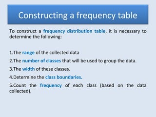
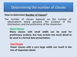
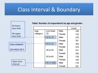
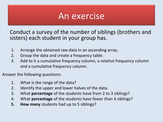
Introduction to Statistics for Built
Environment
Course Code: AED 1222
Compiled by
DEPARTMENT OF ARCHITECTURE AND ENVIRONMENTAL DESIGN (AED)
CENTRE FOR FOUNDATION STUDIES (CFS)
INTERNATIONAL ISLAMIC UNIVERSITY MALAYSIA
Lecture 5
Summarizing Quantitative Data 1
Today’s Lecture:
 Summarizing Quantitative Data:
 The data array
 Frequency Distribution
 Relative Frequency Distribution
 Cumulative Frequency Distribution
Contingency
Table
Contingency
Table
Data
Qualitative Quantitative
TabularTabular GraphicalGraphical TabularTabular GraphicalGraphical
Frequency
Distribution
Frequency
Distribution
Rel. Freq.
Distribution
Rel. Freq.
Distribution
Bar GraphBar Graph
Pie ChartPie Chart
Frequency
Distribution
Frequency
Distribution
Rel. Freq.
Distribution
Rel. Freq.
Distribution
Cumulative
Freq. Dist.
Cumulative
Freq. Dist.
Histograms &
Polygons
Histograms &
Polygons
Stem and
Leaf Plot
Stem and
Leaf Plot
An overview
OgivesOgives
LECTURE
6
LECTURE
4
An overview of common data presentation:
Raw data
Raw data (sometimes called source data or atomic data) is data
that has not been processed for use. A distinction is sometimes
made between data and information to the effect that
information is the end product of data processing.
The simplest way of systematically organizing raw data is the
DATA ARRAY
Although raw data has the potential to become "information," it
requires selective extraction, organization, and sometimes
analysis and formatting for presentation.
The data array
The data array is an arrangement of data items in either an
ascending (from lowest to highest value), or descending (from
highest to lowest value).
The advantages of the data array:
• Identifying the range of data, which is the difference
between the largest and smallest numbers in the data set.
• Identifying the upper and lower halves of the data.
• An array can show the presence of large concentrations of
items at particular values.
In spite of these advantages, the array is an awkward data
organization tool, especially when the number of data items is
very large.
Therefore, there is a need to arrange the data into a more
compact form for analysis and communication purposes.
The data array cont.
Business Statistics: A Decision-
Making Approach, 7e © 2008
Prentice-Hall, Inc.
Example: A manufacturer of insulation randomly selects 20
days and records the daily high temperature.
The data array cont.
DATA
ARRAY
RAW DATA
12, 13, 17, 21, 24, 24, 26, 27, 27, 30, 32, 35, 37, 38, 41, 43, 44, 46, 53, 58
Sort raw data in ascending order:
24, 35, 17, 21, 24, 37, 26, 46, 58, 30,
32, 13, 12, 38, 41, 43, 44, 27, 53, 27
Insulation manufacturer 20 days high temperature record.
Constructing a frequency table
To construct a frequency distribution table, it is necessary to
determine the following:
1.The range of the collected data
2.The number of classes that will be used to group the data.
3.The width of these classes.
4.Determine the class boundaries.
5.Count the frequency of each class (based on the data
collected).
Determining the number of classes
Few Classes
Fewer classes with a very large width can result in the
loss of important detail.
Many Classes
Many classes with small width can be used for
preliminary analysis, but may contain too much detail to
be used in a formal data presentation.
How to determine Number of Classes?
The number of classes depends on the number of
observations being grouped, the purpose of the
distribution, and the preference of the researcher.
In formal presentations, the number of classes used to group the
data generally varies from 5 to 20.
Determining the number of classes cont.
The key is to use classes that give you a good view of the data
pattern and enable you to gain insights into the information
that is there.
• Therefore, the researcher had to determine the suitable
number of classes that suits best to its study.
Business Statistics: A Decision-
Making Approach, 7e © 2008
Prentice-Hall, Inc.
General Guidelines
Number of Data Points Number of Classes
under 50 5 - 7
50 – 100 6 - 10
100 – 250 7 - 12
over 250 10 - 20
– Class widths can typically be reduced as the
number of observations increases
– Distributions with numerous observations are
more likely to be smooth and have gaps filled
since data are plentiful
Determining the number of classes cont.
Determining class interval
Class Interval must satisfy two conditions:
1. All data items from the smallest to the largest must be
included.
2. Each item must be assigned to only one class, i.e. no gaps or
overlapping among classes.
The width of each class (the class interval) should be equal.
To determine the interval of each class, divide the range (the
difference between the highest and lowest items in the data
set) by the desired number of classes, and then round up.
How to determine Class Interval?
Business Statistics: A Decision-
Making Approach, 7e © 2008
Prentice-Hall, Inc.
• The class width is the distance between the
lowest possible value and the highest
possible value for a frequency class.
 The class width formula is :
Largest Value - Smallest Value
Number of Classes
W =
Determining the class interval cont.
Class Interval & Boundary
25=lower
class limit
34=upper
class limit
Open class
interval
Table: Number of respondents by age and gender.
Class midpoint
(35+44)/2=39.5
Table: Heights of 100 male students at XYZ University.
Includes all measurements
from 62.5in. – 65.5in.
(class boundary)
62.5= lower class boundary
65.5= upper class boundary
Size of class interval
Upper class boundary - Lower class boundary
65.5 – 62.5 = 3
68.5 – 65.5 = 3
Class interval & boundary cont.
Business Statistics: A Decision-
Making Approach, 7e © 2008
Prentice-Hall, Inc.
Back to earlier Example :
Constructing a frequency distribution table cont.
DATA
ARRAY
12, 13, 17, 21, 24, 24, 26, 27, 27, 30, 32, 35, 37, 38, 41, 43, 44, 46, 53, 58
Sorted raw data from low to high:
Then….
1.Find range: 58 - 12 = 46
2.Select number of classes: 5 (usually between 5 and 20)
3.Compute class width: 10 (46/5 then round up)
4.Determine class boundaries: 10, 20, 30, 40, 50, 60.
(Sometimes class midpoints are reported: 15, 25, 35, 45, 55)
5.Count the number of values in each class
Insulation manufacturer 20 days high temperature record.
Classes : 5
Width : 10
Example (Cont.):
DATA
ARRAY
12, 13, 17, 21, 24, 24, 26, 27, 27, 30, 32, 35, 37, 38, 41, 43, 44, 46, 53, 58
Constructing a frequency distribution table cont.
Sorted raw data from low to high:
Business Statistics: A Decision-
Making Approach, 7e © 2008
Prentice-Hall, Inc.
Insulation manufacturer 20 days high temperature record.
Why use Frequency Distribution?
• Frequency distribution tables provide insights about
the data that cannot be quickly obtained by looking
only at the original data (raw data).
• In addition, it is a method of organizing data items
into a compact form without obscuring (covering)
essential facts.
• This purpose is achieved by grouping the data into a
relatively small number of classes.
• Therefore, a frequency distribution (for quantitative
data) groups data items into classes and then
records the number of items that appear in each
class.
Frequency Distribution
Relative frequency
Why use Relative Frequency?
• The relative frequency of a class is the fraction or
proportion of the total number of data items
belonging to the class.
• A relative frequency distribution is a tabular summary
of a set of data showing the relative frequency for
each class.
• Relative frequencies can be written as fractions,
percents, or decimals.
Cumulative frequency
What is a Cumulative frequency?
• Cumulative frequency analysis is the analysis of the
frequency of occurrence of values of a phenomenon
less than a reference value.
• i.e. It tells how often the value of the random variable
is less than or equal to a particular reference value.
Surfing time
(minutes)
No. of students
(frequency)
Cumulative
frequency
Relative
frequency
Percentage
300-399 14 14 + 0 = 14 14/400 = 0.035 3.5
400-499 46 14 + 46 = 60 46/400 = 0.115 11.5
500-599 58 60 + 58 = 118 58/400 = 0.145 14.5
600-699 76 118 + 76 = 194 76/400 = 0.19 19.0
700-799 68 194 + 68 = 262 68/400 = 0.17 17.0
800-899 62 262 + 62 = 324 62/400 = 0.155 15.5
900-999 48 324 + 48 = 372 48/400 = 0.12 12.0
1000-1099 22 372 + 22 = 394 22/400 = 0.055 5.5
1100-1199 6 394 + 6 = 400 6/400 = 0.015 1.5
Cumulative frequency cont.
From the table below,
118 students surfed internet for up to 599 minutes (i.e. 599 minutes or less)
324 students surfed internet for up to 899 minutes (i.e. 899 minutes or less)
We can state that:
Time taken by students to surfed internet .
An exercise
Conduct a survey of the number of siblings (brothers and
sisters) each student in your group has.
1. What is the range of the data?
2. Identify the upper and lower halves of the data.
3. What percentage of the students have from 2 to 3 siblings?
4. What percentage of the students have fewer than 4 siblings?
5. How many students had up to 5 siblings?
Answer the following questions:
1. Arrange the obtained raw data in an ascending array.
2. Group the data and create a frequency table.
3. Add to it a cumulative frequency column, a relative frequency column
and a cumulative frequency column.

Aed1222 lesson 5

  • 1.
    Introduction to Statisticsfor Built Environment Course Code: AED 1222 Compiled by DEPARTMENT OF ARCHITECTURE AND ENVIRONMENTAL DESIGN (AED) CENTRE FOR FOUNDATION STUDIES (CFS) INTERNATIONAL ISLAMIC UNIVERSITY MALAYSIA
  • 2.
    Lecture 5 Summarizing QuantitativeData 1 Today’s Lecture:  Summarizing Quantitative Data:  The data array  Frequency Distribution  Relative Frequency Distribution  Cumulative Frequency Distribution
  • 3.
    Contingency Table Contingency Table Data Qualitative Quantitative TabularTabular GraphicalGraphicalTabularTabular GraphicalGraphical Frequency Distribution Frequency Distribution Rel. Freq. Distribution Rel. Freq. Distribution Bar GraphBar Graph Pie ChartPie Chart Frequency Distribution Frequency Distribution Rel. Freq. Distribution Rel. Freq. Distribution Cumulative Freq. Dist. Cumulative Freq. Dist. Histograms & Polygons Histograms & Polygons Stem and Leaf Plot Stem and Leaf Plot An overview OgivesOgives LECTURE 6 LECTURE 4 An overview of common data presentation:
  • 4.
    Raw data Raw data(sometimes called source data or atomic data) is data that has not been processed for use. A distinction is sometimes made between data and information to the effect that information is the end product of data processing. The simplest way of systematically organizing raw data is the DATA ARRAY Although raw data has the potential to become "information," it requires selective extraction, organization, and sometimes analysis and formatting for presentation.
  • 5.
    The data array Thedata array is an arrangement of data items in either an ascending (from lowest to highest value), or descending (from highest to lowest value). The advantages of the data array: • Identifying the range of data, which is the difference between the largest and smallest numbers in the data set. • Identifying the upper and lower halves of the data. • An array can show the presence of large concentrations of items at particular values.
  • 6.
    In spite ofthese advantages, the array is an awkward data organization tool, especially when the number of data items is very large. Therefore, there is a need to arrange the data into a more compact form for analysis and communication purposes. The data array cont.
  • 7.
    Business Statistics: ADecision- Making Approach, 7e © 2008 Prentice-Hall, Inc. Example: A manufacturer of insulation randomly selects 20 days and records the daily high temperature. The data array cont. DATA ARRAY RAW DATA 12, 13, 17, 21, 24, 24, 26, 27, 27, 30, 32, 35, 37, 38, 41, 43, 44, 46, 53, 58 Sort raw data in ascending order: 24, 35, 17, 21, 24, 37, 26, 46, 58, 30, 32, 13, 12, 38, 41, 43, 44, 27, 53, 27 Insulation manufacturer 20 days high temperature record.
  • 8.
    Constructing a frequencytable To construct a frequency distribution table, it is necessary to determine the following: 1.The range of the collected data 2.The number of classes that will be used to group the data. 3.The width of these classes. 4.Determine the class boundaries. 5.Count the frequency of each class (based on the data collected).
  • 9.
    Determining the numberof classes Few Classes Fewer classes with a very large width can result in the loss of important detail. Many Classes Many classes with small width can be used for preliminary analysis, but may contain too much detail to be used in a formal data presentation. How to determine Number of Classes? The number of classes depends on the number of observations being grouped, the purpose of the distribution, and the preference of the researcher.
  • 10.
    In formal presentations,the number of classes used to group the data generally varies from 5 to 20. Determining the number of classes cont. The key is to use classes that give you a good view of the data pattern and enable you to gain insights into the information that is there. • Therefore, the researcher had to determine the suitable number of classes that suits best to its study.
  • 11.
    Business Statistics: ADecision- Making Approach, 7e © 2008 Prentice-Hall, Inc. General Guidelines Number of Data Points Number of Classes under 50 5 - 7 50 – 100 6 - 10 100 – 250 7 - 12 over 250 10 - 20 – Class widths can typically be reduced as the number of observations increases – Distributions with numerous observations are more likely to be smooth and have gaps filled since data are plentiful Determining the number of classes cont.
  • 12.
    Determining class interval ClassInterval must satisfy two conditions: 1. All data items from the smallest to the largest must be included. 2. Each item must be assigned to only one class, i.e. no gaps or overlapping among classes. The width of each class (the class interval) should be equal. To determine the interval of each class, divide the range (the difference between the highest and lowest items in the data set) by the desired number of classes, and then round up. How to determine Class Interval?
  • 13.
    Business Statistics: ADecision- Making Approach, 7e © 2008 Prentice-Hall, Inc. • The class width is the distance between the lowest possible value and the highest possible value for a frequency class.  The class width formula is : Largest Value - Smallest Value Number of Classes W = Determining the class interval cont.
  • 14.
    Class Interval &Boundary 25=lower class limit 34=upper class limit Open class interval Table: Number of respondents by age and gender. Class midpoint (35+44)/2=39.5
  • 15.
    Table: Heights of100 male students at XYZ University. Includes all measurements from 62.5in. – 65.5in. (class boundary) 62.5= lower class boundary 65.5= upper class boundary Size of class interval Upper class boundary - Lower class boundary 65.5 – 62.5 = 3 68.5 – 65.5 = 3 Class interval & boundary cont.
  • 16.
    Business Statistics: ADecision- Making Approach, 7e © 2008 Prentice-Hall, Inc. Back to earlier Example : Constructing a frequency distribution table cont. DATA ARRAY 12, 13, 17, 21, 24, 24, 26, 27, 27, 30, 32, 35, 37, 38, 41, 43, 44, 46, 53, 58 Sorted raw data from low to high: Then…. 1.Find range: 58 - 12 = 46 2.Select number of classes: 5 (usually between 5 and 20) 3.Compute class width: 10 (46/5 then round up) 4.Determine class boundaries: 10, 20, 30, 40, 50, 60. (Sometimes class midpoints are reported: 15, 25, 35, 45, 55) 5.Count the number of values in each class Insulation manufacturer 20 days high temperature record.
  • 17.
    Classes : 5 Width: 10 Example (Cont.): DATA ARRAY 12, 13, 17, 21, 24, 24, 26, 27, 27, 30, 32, 35, 37, 38, 41, 43, 44, 46, 53, 58 Constructing a frequency distribution table cont. Sorted raw data from low to high: Business Statistics: A Decision- Making Approach, 7e © 2008 Prentice-Hall, Inc. Insulation manufacturer 20 days high temperature record.
  • 18.
    Why use FrequencyDistribution? • Frequency distribution tables provide insights about the data that cannot be quickly obtained by looking only at the original data (raw data). • In addition, it is a method of organizing data items into a compact form without obscuring (covering) essential facts. • This purpose is achieved by grouping the data into a relatively small number of classes. • Therefore, a frequency distribution (for quantitative data) groups data items into classes and then records the number of items that appear in each class. Frequency Distribution
  • 19.
    Relative frequency Why useRelative Frequency? • The relative frequency of a class is the fraction or proportion of the total number of data items belonging to the class. • A relative frequency distribution is a tabular summary of a set of data showing the relative frequency for each class. • Relative frequencies can be written as fractions, percents, or decimals.
  • 20.
    Cumulative frequency What isa Cumulative frequency? • Cumulative frequency analysis is the analysis of the frequency of occurrence of values of a phenomenon less than a reference value. • i.e. It tells how often the value of the random variable is less than or equal to a particular reference value.
  • 21.
    Surfing time (minutes) No. ofstudents (frequency) Cumulative frequency Relative frequency Percentage 300-399 14 14 + 0 = 14 14/400 = 0.035 3.5 400-499 46 14 + 46 = 60 46/400 = 0.115 11.5 500-599 58 60 + 58 = 118 58/400 = 0.145 14.5 600-699 76 118 + 76 = 194 76/400 = 0.19 19.0 700-799 68 194 + 68 = 262 68/400 = 0.17 17.0 800-899 62 262 + 62 = 324 62/400 = 0.155 15.5 900-999 48 324 + 48 = 372 48/400 = 0.12 12.0 1000-1099 22 372 + 22 = 394 22/400 = 0.055 5.5 1100-1199 6 394 + 6 = 400 6/400 = 0.015 1.5 Cumulative frequency cont. From the table below, 118 students surfed internet for up to 599 minutes (i.e. 599 minutes or less) 324 students surfed internet for up to 899 minutes (i.e. 899 minutes or less) We can state that: Time taken by students to surfed internet .
  • 22.
    An exercise Conduct asurvey of the number of siblings (brothers and sisters) each student in your group has. 1. What is the range of the data? 2. Identify the upper and lower halves of the data. 3. What percentage of the students have from 2 to 3 siblings? 4. What percentage of the students have fewer than 4 siblings? 5. How many students had up to 5 siblings? Answer the following questions: 1. Arrange the obtained raw data in an ascending array. 2. Group the data and create a frequency table. 3. Add to it a cumulative frequency column, a relative frequency column and a cumulative frequency column.

Editor's Notes

  • #2 Updated Version 02/11/2011
  • #23 Raw data can be collected from students and written on the board. Then they can be arranged in an ascending array, and then grouped. A suggested grouping is: Less than 2, 2-3, 4-5, more than 5. The answers to questions 1 & 2 are derived from the array. The answer to questions 3, 4 & 5 are derived from the frequency table.