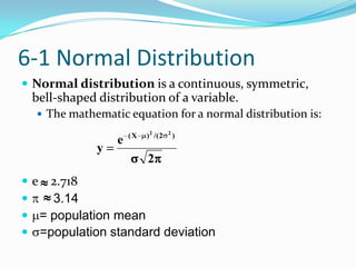
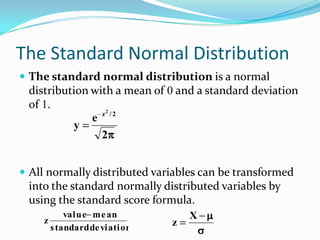
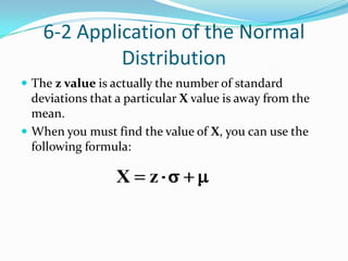
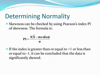
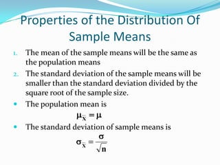
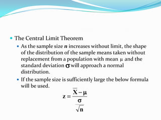
Statistics
6-1 Normal Distribution
 Normal distribution is a continuous, symmetric,
 bell-shaped distribution of a variable.
   The mathematic equation for a normal distribution is:

                     (X   ) 2 /( 2   2
                                         )
                 e
             y
                          2
 e 2.718
   3.14
 = population mean
 =population standard deviation
Properties of the Theoretical
               Distribution
1. A normal distribution is bell-shaped.
2. The mean, median, and mode are equal and are
   located at the center of the distribution.
3. A normal distribution curve is unimodal.
4. The curve is symmetric about the mean, which is
   equivalent to saying its shape is the same on both
   sides of a vertical line passing through the center.
5. The curve is continuous; that is, there are no gaps or
   holes. For each value of X, there is a corresponding value
   of Y.
6. The curve never touches the x axis. Theoretically, no
   matter how far in either direction the curve extends, it
   never meets the x axis-but it gets increasingly closer.
7. The total area under a normal distribution curve is equal
   to 1.00, or 100%.
8. The area under the part of a normal curve that lies within
   1 standard deviation of the mean is approx. 68%; within 2
   standard deviations, about 95%; and within 3 standard
   deviations, about 99.7%.
The Standard Normal Distribution
 The standard normal distribution is a normal
 distribution with a mean of 0 and a standard deviation
 of 1.
                z2 / 2
              e
          y
                2


 All normally distributed variables can be transformed
 into the standard normally distributed variables by
 using the standard score formula.
            value m e an           X
    z                          z
        s tandard de viation
6-2 Application of the Normal
             Distribution
 The z value is actually the number of standard
  deviations that a particular X value is away from the
  mean.
 When you must find the value of X, you can use the
  following formula:

                  X     z
Determining Normality
 Skewness can be checked by using Pearson’s index PI
  of skewness. The formula is:

                3( X me dian
                           )
           PI


 If the index is greater than or equal to +1 or less than
  or equal to -1, it can be concluded that the data is
  significantly skewed.
6-3 The Central Limit Theorem
 A sampling distribution of the sample means is a
  distribution using the means computed from all
  possible random samples of a specific size taken from a
  population.
 Sampling error is the difference between the sample
  measure and the corresponding population measure
  due to the fact that the sample is not a perfect
  representation of the population.
Properties of the Distribution Of
             Sample Means
1. The mean of the sample means will be the same as
   the population means
2. The standard deviation of the sample means will be
   smaller than the standard deviation divided by the
   square root of the sample size.
 The population mean is
                     X
     The standard deviation of sample means is

                     X
                           n
 The Central Limit Theorem
    As the sample size n increases without limit, the shape
     of the distribution of the sample means taken without
     replacement from a population with mean and the
     standard deviation will approach a normal
     distribution.
    If the sample size is sufficiently large the below formula
     will be used.
                            X
                        z

                                n
6-4 The Normal Approximation to
the Binomial Distribution
 A correction for continuity is a correction employed
 when a continuous distribution is used to approximate
 a discrete distribution.

                    n p
                      n p q

The Normal Distribution

  • 1.
  • 2.
    6-1 Normal Distribution Normal distribution is a continuous, symmetric, bell-shaped distribution of a variable.  The mathematic equation for a normal distribution is: (X ) 2 /( 2 2 ) e y 2  e 2.718  3.14  = population mean  =population standard deviation
  • 3.
    Properties of theTheoretical Distribution 1. A normal distribution is bell-shaped. 2. The mean, median, and mode are equal and are located at the center of the distribution. 3. A normal distribution curve is unimodal. 4. The curve is symmetric about the mean, which is equivalent to saying its shape is the same on both sides of a vertical line passing through the center.
  • 4.
    5. The curveis continuous; that is, there are no gaps or holes. For each value of X, there is a corresponding value of Y. 6. The curve never touches the x axis. Theoretically, no matter how far in either direction the curve extends, it never meets the x axis-but it gets increasingly closer. 7. The total area under a normal distribution curve is equal to 1.00, or 100%. 8. The area under the part of a normal curve that lies within 1 standard deviation of the mean is approx. 68%; within 2 standard deviations, about 95%; and within 3 standard deviations, about 99.7%.
  • 5.
    The Standard NormalDistribution  The standard normal distribution is a normal distribution with a mean of 0 and a standard deviation of 1. z2 / 2 e y 2  All normally distributed variables can be transformed into the standard normally distributed variables by using the standard score formula. value m e an X z z s tandard de viation
  • 6.
    6-2 Application ofthe Normal Distribution  The z value is actually the number of standard deviations that a particular X value is away from the mean.  When you must find the value of X, you can use the following formula: X z
  • 7.
    Determining Normality  Skewnesscan be checked by using Pearson’s index PI of skewness. The formula is: 3( X me dian ) PI  If the index is greater than or equal to +1 or less than or equal to -1, it can be concluded that the data is significantly skewed.
  • 8.
    6-3 The CentralLimit Theorem  A sampling distribution of the sample means is a distribution using the means computed from all possible random samples of a specific size taken from a population.  Sampling error is the difference between the sample measure and the corresponding population measure due to the fact that the sample is not a perfect representation of the population.
  • 9.
    Properties of theDistribution Of Sample Means 1. The mean of the sample means will be the same as the population means 2. The standard deviation of the sample means will be smaller than the standard deviation divided by the square root of the sample size.  The population mean is X  The standard deviation of sample means is X n
  • 10.
     The CentralLimit Theorem  As the sample size n increases without limit, the shape of the distribution of the sample means taken without replacement from a population with mean and the standard deviation will approach a normal distribution.  If the sample size is sufficiently large the below formula will be used. X z n
  • 11.
    6-4 The NormalApproximation to the Binomial Distribution  A correction for continuity is a correction employed when a continuous distribution is used to approximate a discrete distribution. n p n p q