Anova by Hazilah Mohd Amin

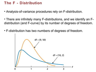
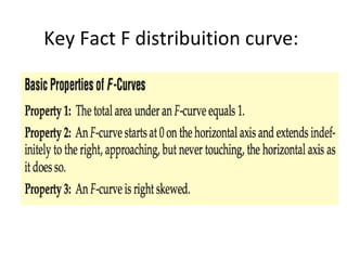
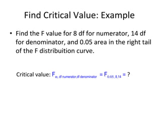
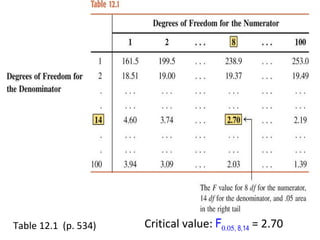
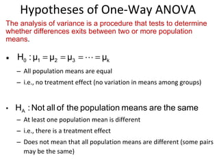
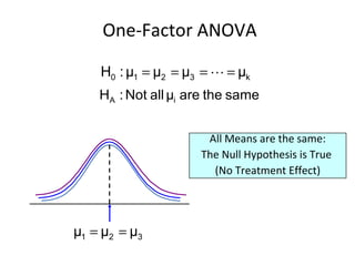
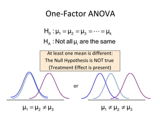
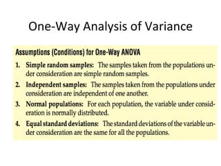
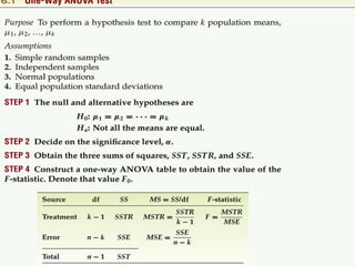
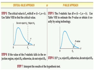
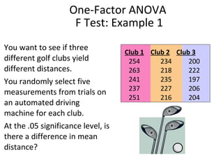
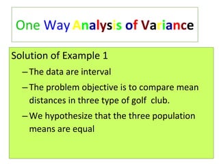
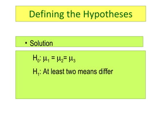
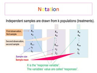
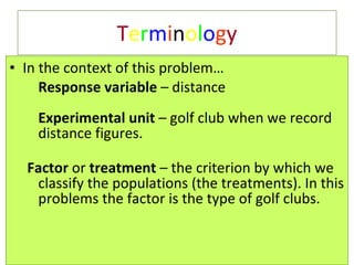
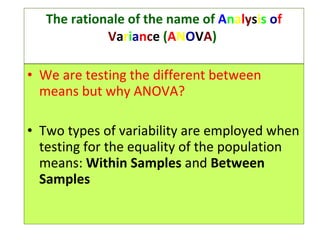
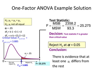
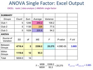
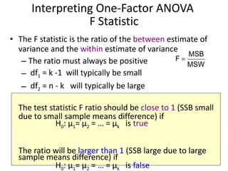
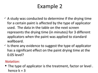
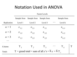
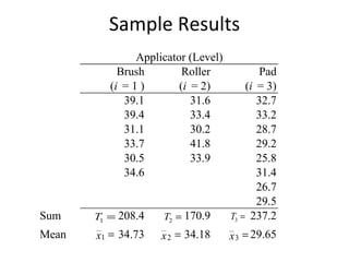
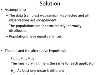
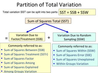
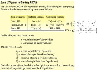
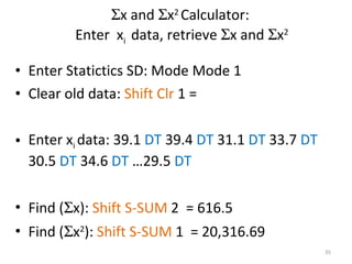
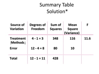
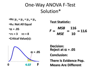
Hazilah Mohd Amin Analysis of Variance (ANOVA)

Goals After completing, you should be able to: Recognize situations in which to use analysis of variance (ANOVA) Perform a single-factor hypothesis test for Comparing More Than Two Means and interpret results

The F - Distribution Analysis-of-variance procedures rely on F-distribution. There are infinitely many F-distributions, and we identify an F-distribution (and F-curve) by its number of degrees of freedom. F-distribution has two numbers of degrees of freedom.

Key Fact F distribuition curve:

Find Critical Value: Example Find the F value for 8 df for numerator, 14 df for denominator, and 0.05 area in the right tail of the F distribuition curve. Critical value: F  , df numerator,df denominator = F  , 8,14 = ?

Table 12.1 (p. 534) Critical value: F  , 8,14 = 2.70

Hypotheses of One-Way ANOVA All population means are equal i.e., no treatment effect (no variation in means among groups) At least one population mean is different i.e., there is a treatment effect Does not mean that all population means are different (some pairs may be the same) The analysis of variance is a procedure that tests to determine whether differences exits between two or more population means .

One-Factor ANOVA All Means are the same: The Null Hypothesis is True (No Treatment Effect)

One-Factor ANOVA At least one mean is different: The Null Hypothesis is NOT true (Treatment Effect is present) or

One-Factor ANOVA F Test: Example 1 You want to see if three different golf clubs yield different distances. You randomly select five measurements from trials on an automated driving machine for each club. At the .05 significance level, is there a difference in mean distance? Club 1 Club 2 Club 3 254 234 200 263 218 222 241 235 197 237 227 206 251 216 204

Solution of Example 1 The data are interval The problem objective is to compare mean distances in three type of golf club. We hypothesize that the three population means are equal One Way A n a l y s i s o f V a r i a n c e

Defining the Hypotheses H 0 :  1 =  2 =  3 H 1 : At least two means differ Solution

N o t a t i o n Independent samples are drawn from k populations (treatments). X 11 x 21 . . . X n1,1 X 12 x 22 . . . X n2,2 X 1k x 2k . . . X nk,k Sample size Sample mean X is the “response variable”. The variables’ value are called “responses”.

T e r m i n o l o g y In the context of this problem… Response variable – distance Experimental unit – golf club when we record distance figures. Factor or treatment – the criterion by which we classify the populations (the treatments). In this problems the factor is the type of golf clubs.

The rationale of the name of A n a l y s i s o f V a r i a n c e ( A N O V A ) We are testing the different between means but why ANOVA? Two types of variability are employed when testing for the equality of the population means: Within Samples and Between Samples

One Way A n a l y s i s o f V a r i a n c e Graphical demonstration : Employing two types of variability: Within Samples and Between Samples

Treatment 1 Treatment 2 Treatment 3 20 16 15 14 11 10 9 The sample means are the same as before, but the larger within-sample variability makes it harder to draw a conclusion about the population means. A small variability within the samples makes it easier to draw a conclusion about the population means. 20 25 30 1 7 Treatment 1 Treatment 2 Treatment 3 10 12 19 9

One-Factor ANOVA Example: Scatter Diagram • • • • • 270 260 250 240 230 220 210 200 190 • • • • • • • • • • Distance Club 1 Club 2 Club 3 254 234 200 263 218 222 241 235 197 237 227 206 251 216 204 Club 1 2 3 From scatter diagram, we can clearly see sample means difference because of small within-sample variability

Test Statistics (F), Critical Value & Rejection Criterion Test statistic: where MSB is mean squares between variances where MSW is mean squares within variances Rejection Region: F > F  , k-1,n-k Degrees of freedom df 1 = k – 1 (k = levels or treatments) df 2 = n – k (n = sum of sample sizes from all populations) H 0 : μ 1 = μ 2 = … = μ k H A : At least two population means are different The hypothesis test:

One-Factor ANOVA Example Computations Club 1 Club 2 Club 3 254 234 200 263 218 222 241 235 197 237 227 206 251 216 204 x 1 = 249.2 x 2 = 226.0 x 3 = 205.8 x = 227.0 n 1 = 5 n 2 = 5 n 3 = 5 n = 15 k = 3 MSB = 4716.4 / (3-1) = 2358.2 MSW = 1119.6 / (15-3) = 93.3 SSB = 4716.4 SSW = 1119.6

One-Factor ANOVA Example Solution H 0 : μ 1 = μ 2 = μ 3 H A : μ i not all equal  = .05 df 1 = k-1 =3-1 =2 df 2 = n-k =15-3 =12 F = 25.275 Test Statistic: Decision: Test statistic F is greater than critical value Conclusion: Reject H 0 at  = 0.05 There is evidence that at least one μ i differs from the rest 0  = .05 F .05 = 3.885 Reject H 0 Do not reject H 0 Critical Value: F  , k-1,n-k = F  , 2,12 = 3.885

ANOVA Single Factor: Excel Output EXCEL: tools | data analysis | ANOVA: single factor F  , k-1,n-k = F  , 2,12 = 3.885 SUMMARY Groups Count Sum Average Variance Club 1 5 1246 249.2 108.2 Club 2 5 1130 226 77.5 Club 3 5 1029 205.8 94.2 ANOVA Source of Variation SS df MS F P-value F crit Between Groups 4716.4 2 2358.2 25.275 4.99E-05 3.885 Within Groups 1119.6 12 93.3 Total 5836.0 14

Rationale 1: Variability Between Sample If H 0 : μ 1 = μ 2 = … = μ k is true , we would expect all the sample means to be close to one another. If the alternative hypothesis is true, at least some of the sample means would differ. Thus, we measure variability between sample means (and hence MSB or MSTr).

Large variability within the samples weakens the “ability” of the sample means to represent their corresponding population means. Therefore, even though sample means may markedly differ from one another, we have to consider the “within samples variability” (and hence MSW or MSE). Rationale II: Variability Within

Interpreting One-Factor ANOVA F Statistic The F statistic is the ratio of the between estimate of variance and the within estimate of variance The ratio must always be positive df 1 = k -1 will typically be small df 2 = n - k will typically be large The test statistic F ratio should be close to 1 (SSB small due to small sample means difference) if H 0 : μ 1 = μ 2 = … = μ k is true The ratio will be larger than 1 (SSB large due to large sample means difference) if H 0 : μ 1 = μ 2 = … = μ k is false

Example 2 A study was conducted to determine if the drying time for a certain paint is affected by the type of applicator used. The data in the table on the next screen represents the drying time (in minutes) for 3 different applicators when the paint was applied to standard wallboard. Is there any evidence to suggest the type of applicator has a significant effect on the paint drying time at the 0.05 level? Notation : The type of applicator is the treatment, factor or level . hence k = 3

Notation Used in ANOVA Factor Levels Sample from Sample from Sample from Sample from Replication Level 1 Level 2 Level 3 Level k n = 1 x 1,1 x 2,1 x 3,1 x k ,1 n = 2 x 1,2 x 2,2 x 3,2 x k ,2 n = 3 x 1,3 x 2,3 x 3,3 x k ,3 Column T 1 T 2 T 3 T k T Totals T = grand total = sum of all x 's =  x =  T i . . . . . . . . .

Sample Results  1 x  2 x  3 x

Solution Assumptions: The data (samples) was randomly collected and all observations are independent. The populations are (approximately) normally distributed. Populations have equal variances. The null and the alternative hypothesis: H o :  1 =  2 =  3 The mean drying time is the same for each applicator H a : At least one mean is different Not all drying time means are equal

Partition of Total Variation Commonly referred to as: Sum of Squares Within (SSW) Sum of Squares Error (SSE) Sum of Squares Unexplained Within Groups Variation Variation Due to Factor/Treatment (SSB) Variation Due to Random Sampling (SSW) Sum of Squares Total (SST) Commonly referred to as: Sum of Squares Between (SSB) Sum of Squares Treatment (SSTr) Sum of Squares Factor Sum of Squares Among Sum of Squares Explained Among Groups Variation = + Total variation SST can be split into two parts: SST = SSB + SSW

 x and  x 2 Calculator: Enter x i data, retrieve  x and  x 2 Enter Statictics SD: Mode Mode 1 Clear old data: Shift Clr 1 = Enter x i data: 39.1 DT 39.4 DT 31.1 DT 33.7 DT 30.5 DT 34.6 DT …29.5 DT Find (  x): Shift S-SUM 2 = 616.5 Find (  x 2 ): Shift S-SUM 1 = 20,316.69

Mean Square The mean square for the factor being tested and for the error is obtained by dividing the sum-of-square value by the corresponding number of degrees of freedom Numerator degrees of freedom = df(factor) = k  1 = 3  1 = 2 df(total) = n  1 = 19  1 = 18 Denominator degrees of freedom = df(error) = n  k = 19  3 = 16 Calculations:

One-Way ANOVA Table Source of Variation df SS MS Between Samples SSB MSB = Within Samples n - k SSW MSW = Total n - 1 SST = SSB+SSW k - 1 MSB MSW F ratio SSB k - 1 SSW n - k F = The sums of squares and the degrees of freedom must check SS(factor) + SS(error) = SS(total) or SSB + SSW = SST df(factor) + df(error) = df(total) or df(between) + df(within) = df(total) An ANOVA table is often used to record the sums of squares and to organize the rest of the calculations. Format for the ANOVA Table:

The Completed ANOVA Table The Complete ANOVA Table: The Test Statistic:

Solution Continued The Results a. Decision: Reject H o at  = 0.05 b. Conclusion : There is evidence to suggest the three population means are not all the same. The type of applicator has a significant effect on the paint drying time at the 0.05 level of significance. Critical Value: F  , k-1,n-k = F  , 2,16 = 3.63 The Test Statistic F = 4.27 is in the rejection region. Reject H 0 F .05 = 3.63 Do not reject H 0  = .05

One-Way ANOVA F-Test: Exercise 1 You’re a trainer for Microsoft Corp. Is there any evidence to suggest the type of training method has a significant effect on the learning time at the 0.05 level? The data in the table represents the learning times (in hours) of 12 people using 4 different training methods. M1 M2 M3 M4 10 11 13 18 9 16 8 23 5 9 9 25 © 1984-1994 T/Maker Co. Answer: Critical Value = 4.07. Test statistic = 11.6

Hey! Lets get our hand dirty … Using S P S S ….

One Way A n a l y s i s o f V a r i a n c e U s i n g S P S S Suppose we want to know whether students who have to work many hours outside school to support themselves find their grade suffering. We examine this question by comparing the GPAs of students who work various hours outside school. Let’s examine this question using data in Student file. File>Open> Student

One Way A n a l y s i s o f V a r i a n c e U s i n g S P S S First examine the average GPA for each of the three work categories (0 hrs, 1-19hrs, >20hrs) - WorkCat Graph > Boxplot then choose Simple and click Define . Select GPA as the variable and WorkCat for the Category Axis. Click Option

After Clicking Options …, click off Display groups defined by missing value , and click Continue then OK . You’ll get this

What is the Box-plot telling us? Some variation across the groups See median GPAs (dark line in the middle of box) differ slightly between groups. So, should we attribute the observed difference to sampling error or they genuinely differ? Neither box-plot nor the median offer decisive evidence. Hence we need ANOVA.

One Way A n a l y s i s o f V a r i a n c e U s i n g S P S S We are testing: H 0 :  1 =  2 =  3 H 1 : At least two means differ Before attempting ANOVA, need to review the ANOVA assumptions. Independent samples (ii) Normality (iii) Variances equality. We can test both (ii) & (iii). Analyze>Descriptive Statistics>Explore

Analyze>Descriptive Statistics>Explore In the Explore dialog box, select GPAs as the dependent List variable, WorkCat as the Factor List variable and Plot as the Display . Next, click Plot … We are interested in a normality test, select Select this & deselect this only. Click Continue and OK . See next slide…

The Output has several parts, let focus on the tests of normality The Kolmogorov-Smirnov test assesses whether there is significant departure from normality in the population distribution of the 3 groups. H 0 : Distributions are normal . Look at the p-values, all are > 0.05. Do not reject H 0 . Hence no evidence of non-normality.

One Way A n a l y s i s o f V a r i a n c e U s i n g S P S S We still need to validate the homogeneity of variance assumption. We do this within ANOVA. Analyze>Compare Means>One-Way ANOVA Dependent List variable is GPA and Factor variable is WorkCat. Click Option,

One Way A n a l y s i s o f V a r i a n c e U s i n g S P S S under Statistics , select Descriptive and Homogeneity of variance test . Click Continue & OK H 0 : Variances are equal. One-Way ANOVA output consists many parts. Look at the p-value > 0.05. Hence do not reject H 0 .

Normality & Homogeneity of variances assumptions met … hence Let find out whether students who work various hours outside school differ in their GPAs. The P-value of .000 is very small, hence we reject Ho and conclude that the means GPAs are not all the same. Where are the differences? Hence Post-Hoc test…

One-Way ANOVA F-Test: Exercise 1 Solution You’re a trainer for Microsoft Corp. Is there any evidence to suggest the type of training method has a significant effect on the learning time at the 0.05 level? The data in the table represents the learning times (in hours) of 12 people using 4 different training methods. M1 M2 M3 M4 10 11 13 18 9 16 8 23 5 9 9 25 © 1984-1994 T/Maker Co.

Summary Table Solution* Source of Variation Degrees of Freedom Sum of Squares Mean Square (Variance) F Treatment ( Methods ) 4 - 1 = 3 348 116 11.6 Error 12 - 4 = 8 80 10 Total 12 - 1 = 11 428

One-Way ANOVA F-Test Solution* H 0 :  1 =  2 =  3 =  4 H a : Not All Equal  = .05  1 = 3  2 = 8 Critical Value(s): F 0 4.07 Test Statistic: Decision: Conclusion: Reject at  = .05 There Is Evidence Pop. Means Are Different  = .05 F MSB MSE    116 10 11 6 .

Anova by Hazilah Mohd Amin

In this document