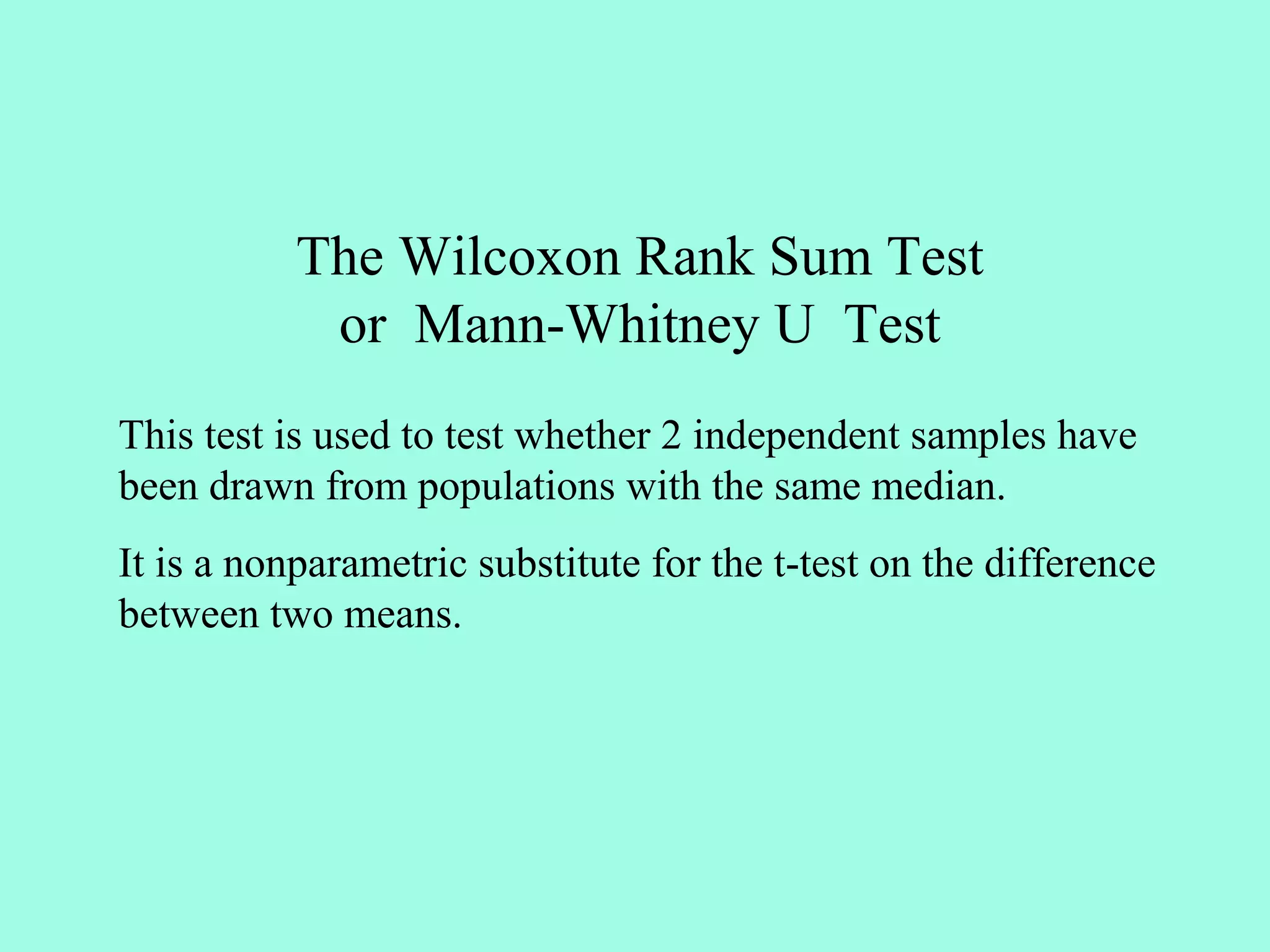
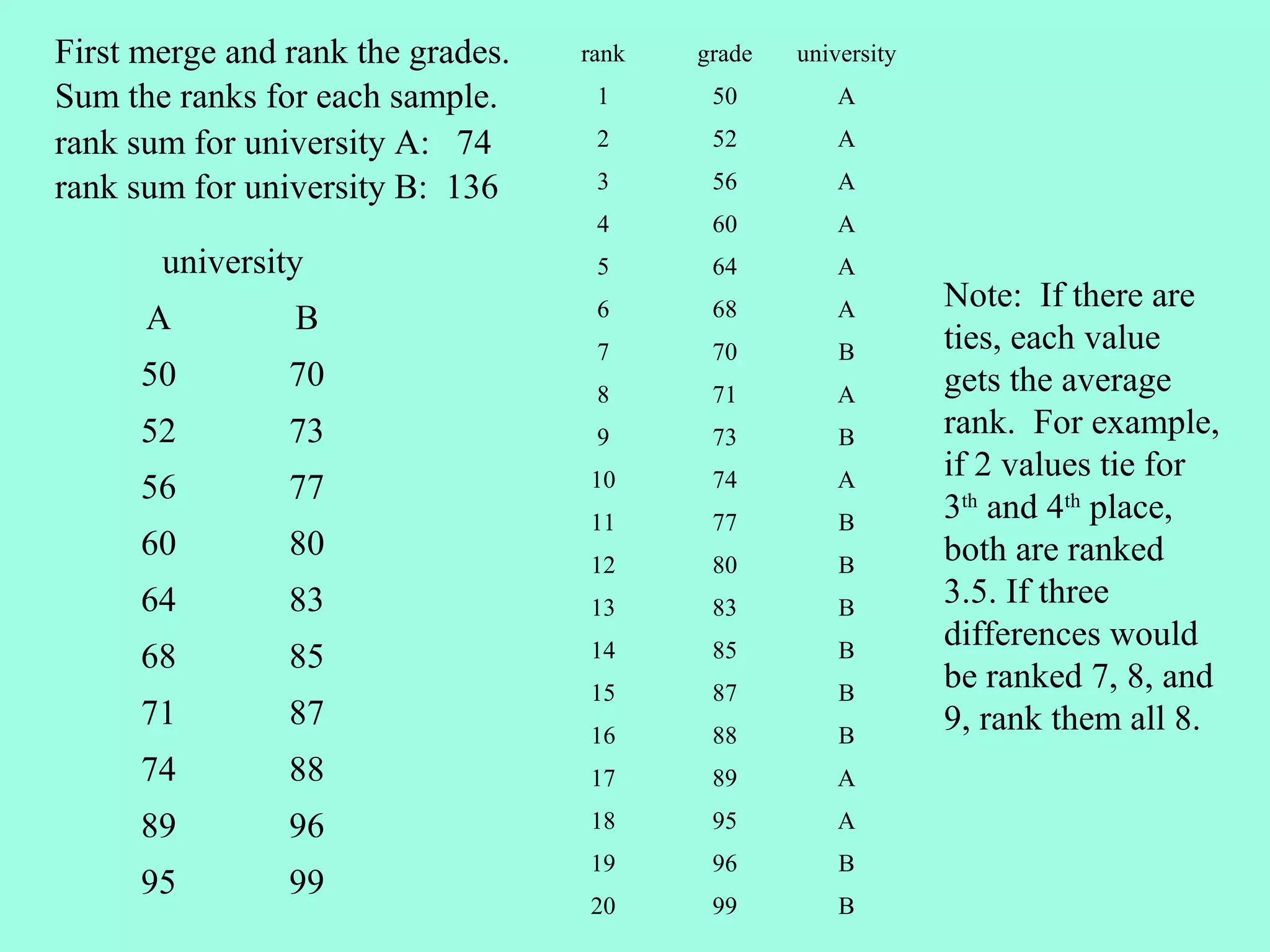
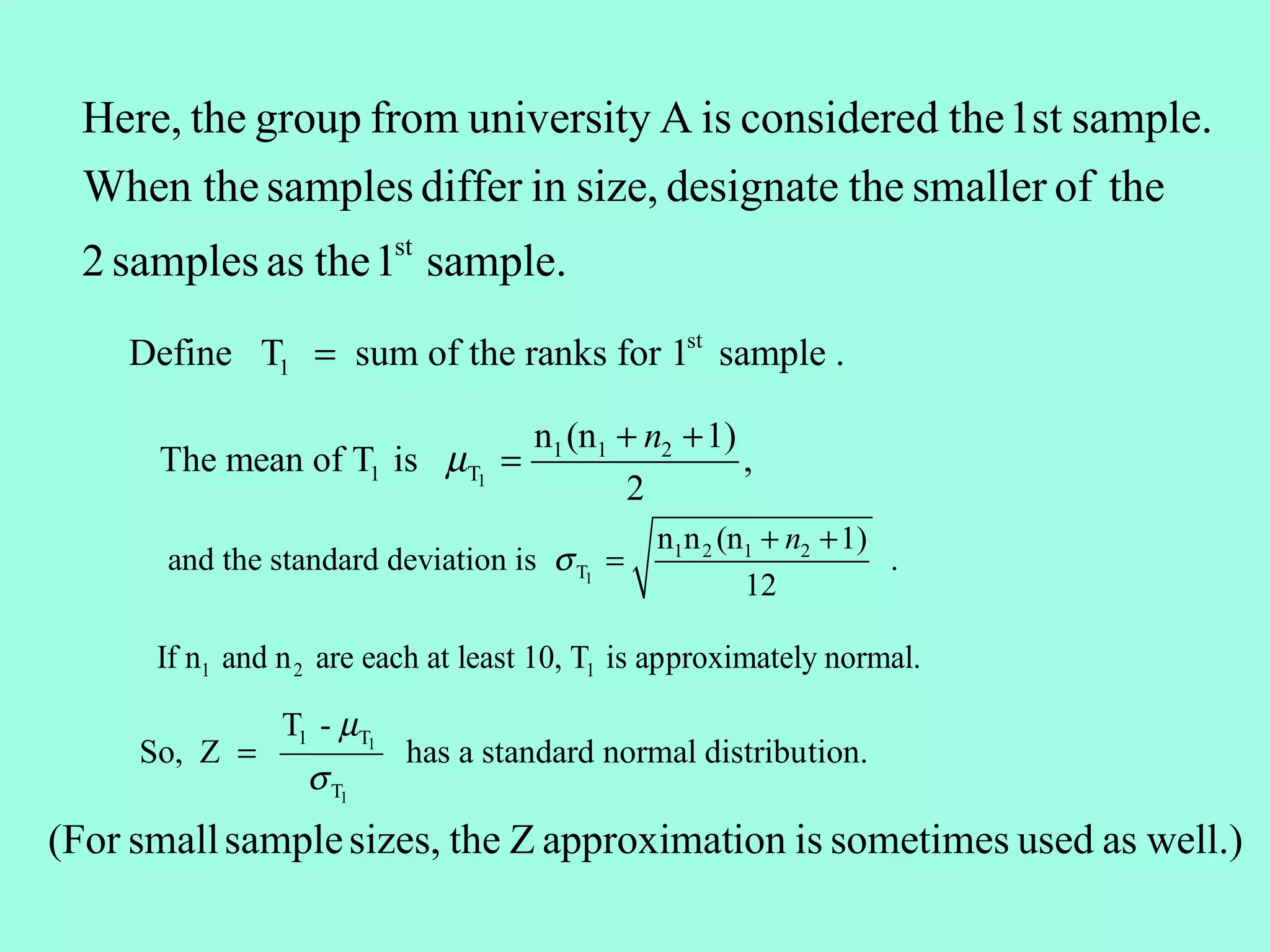
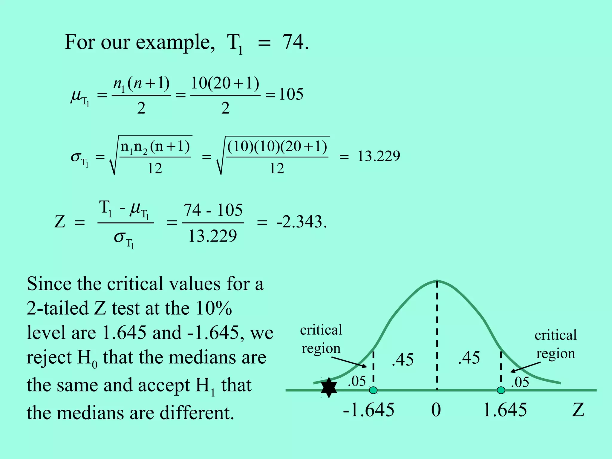
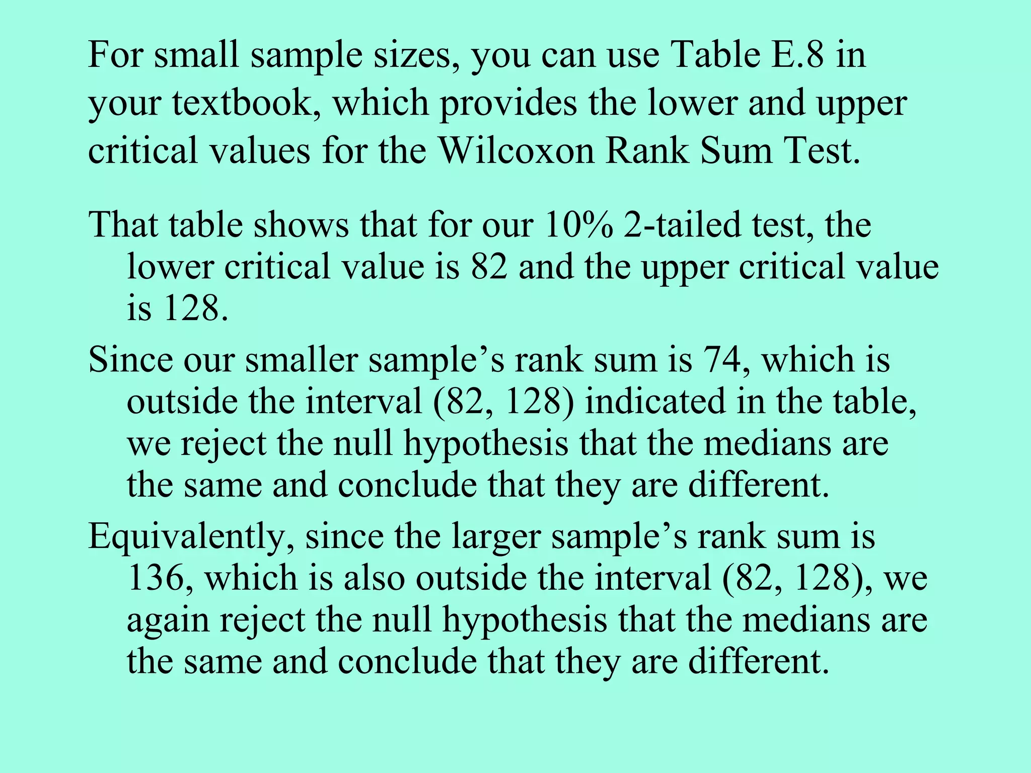
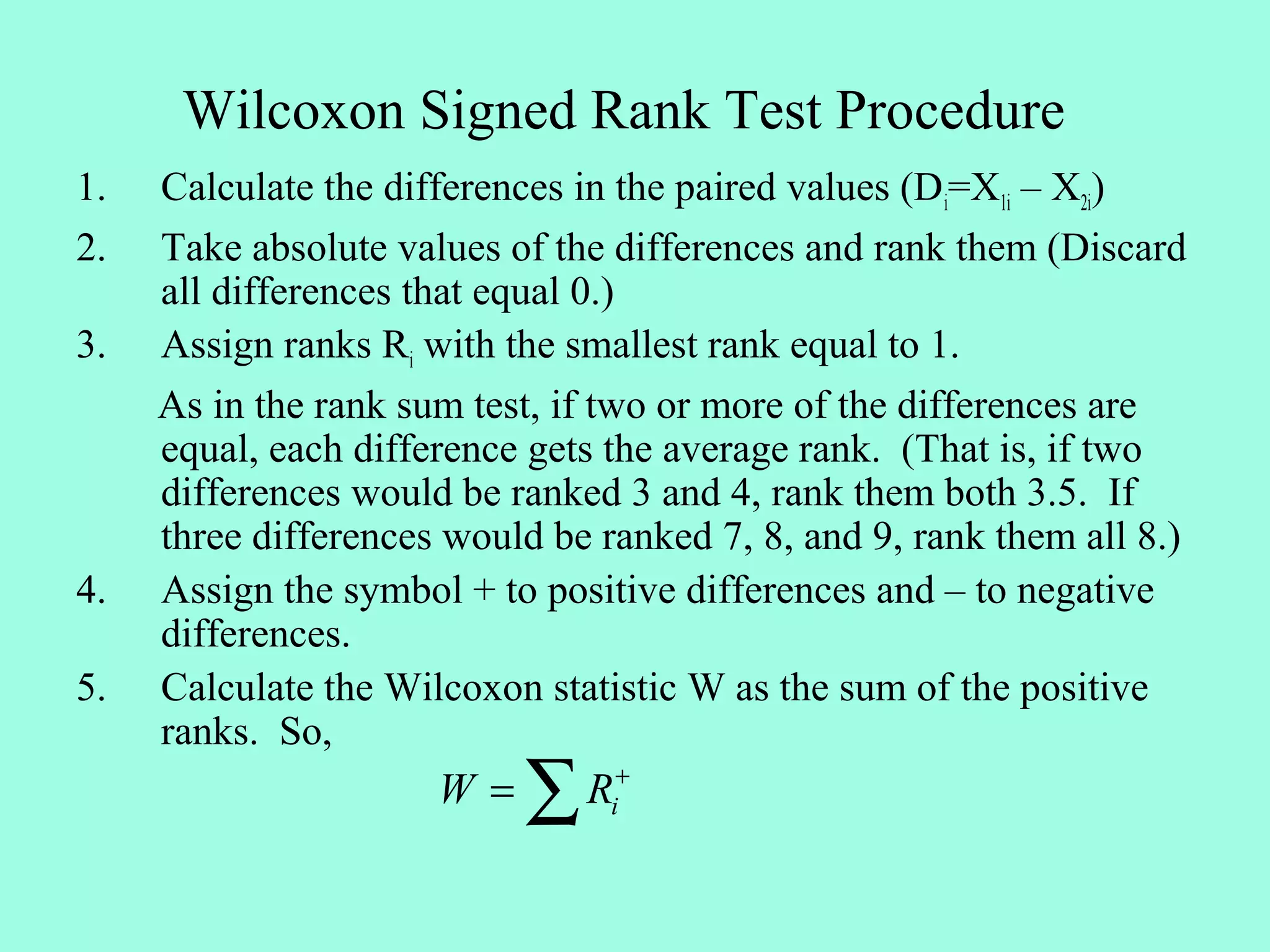
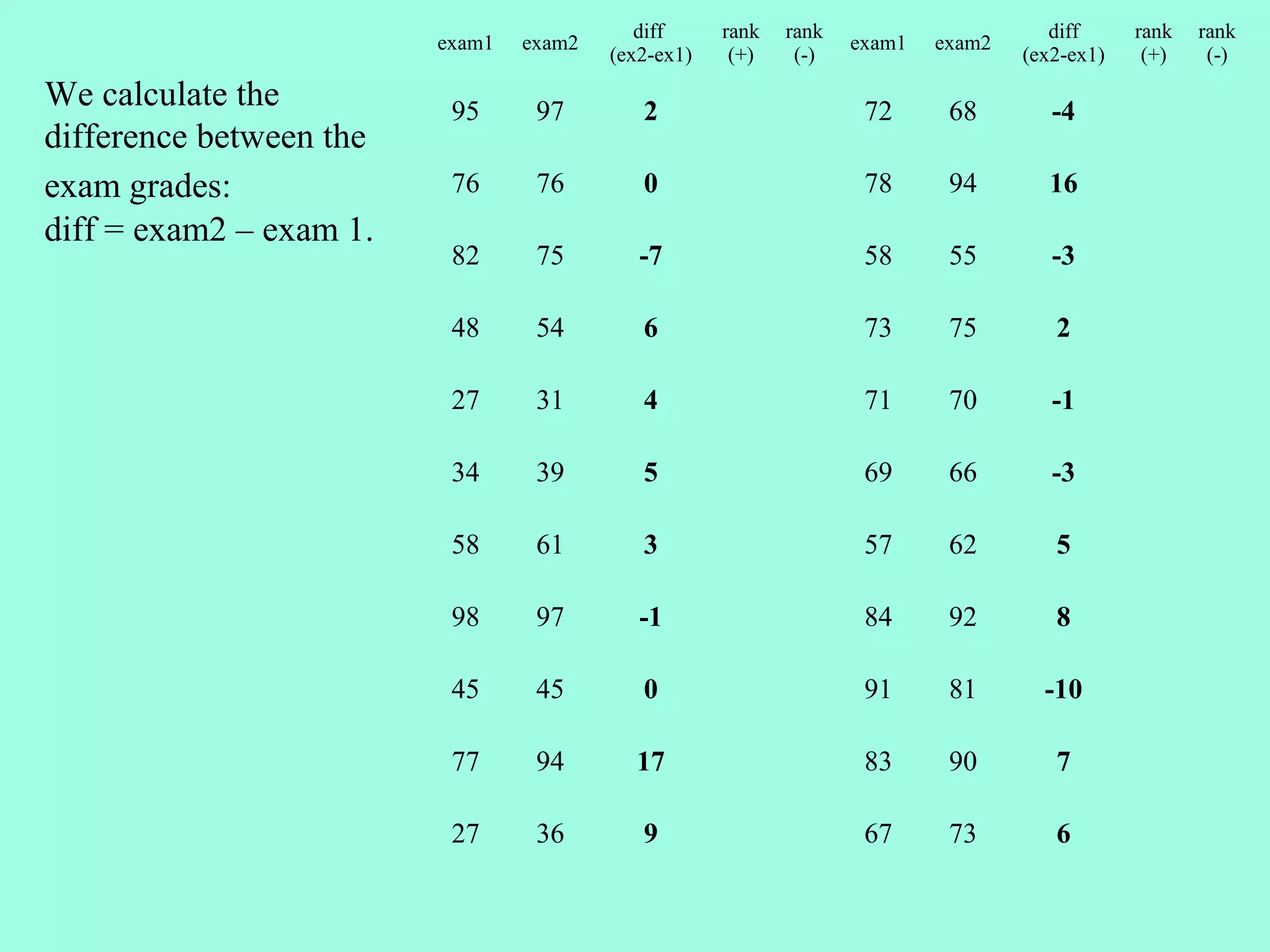
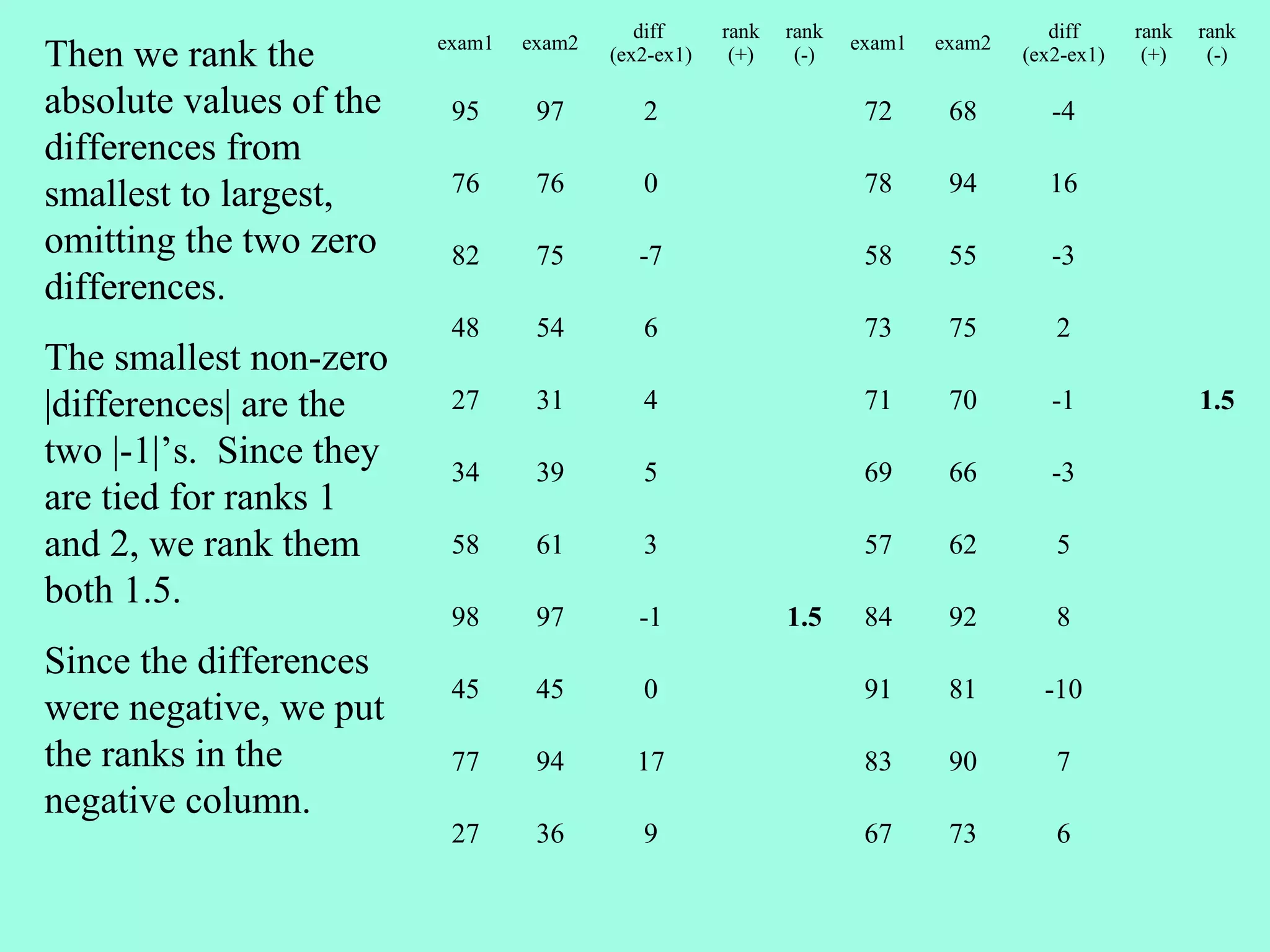
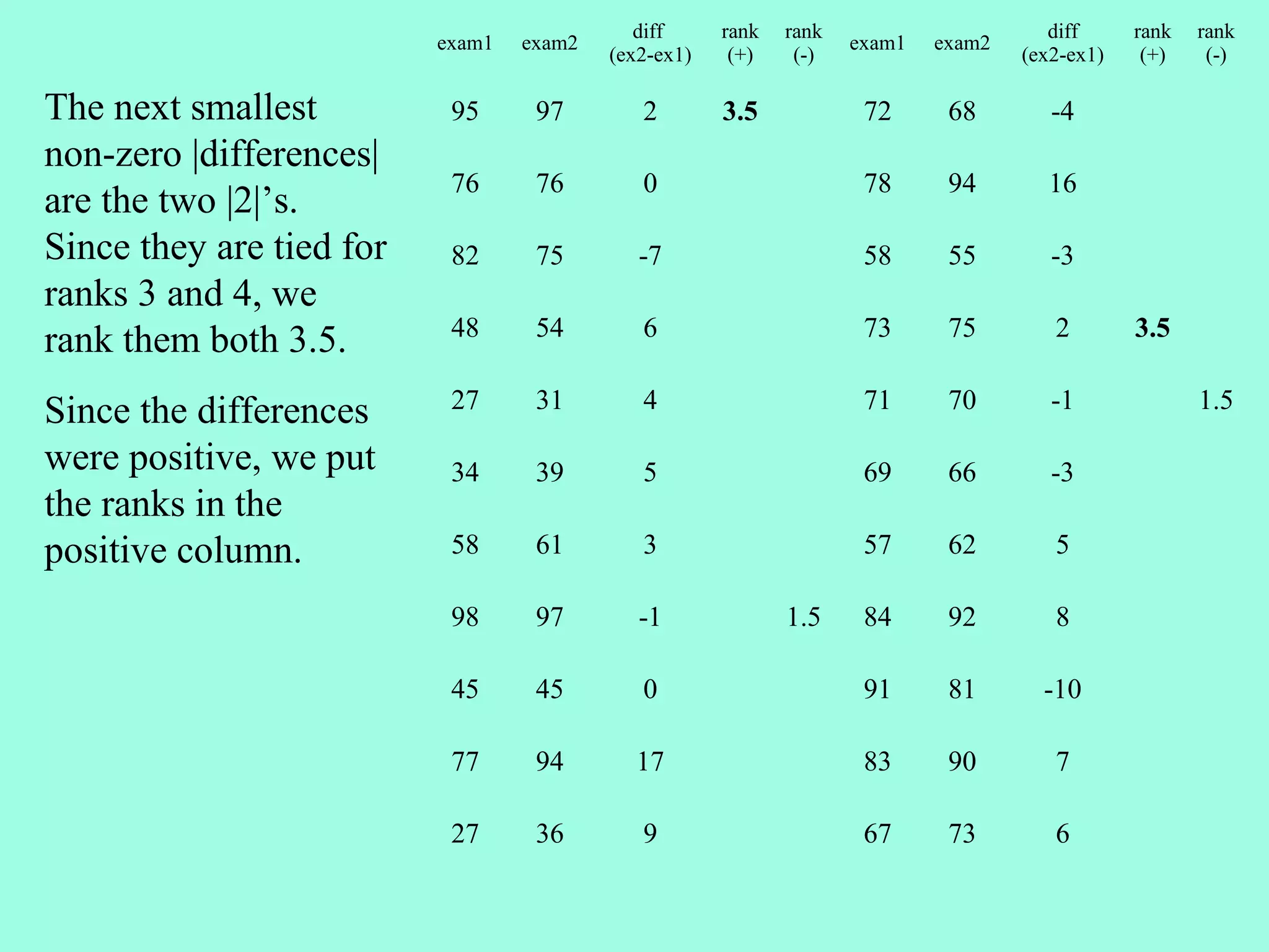
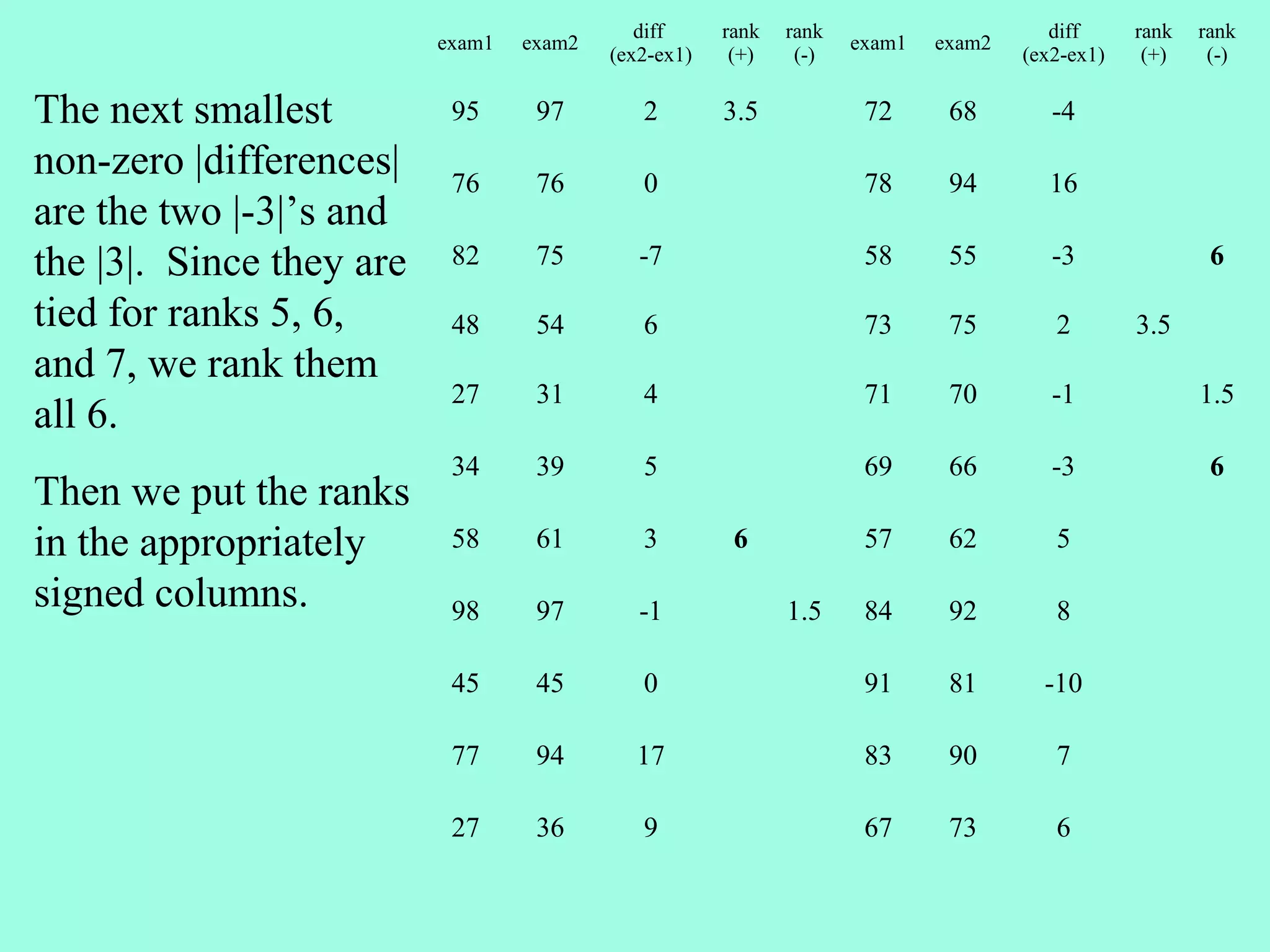
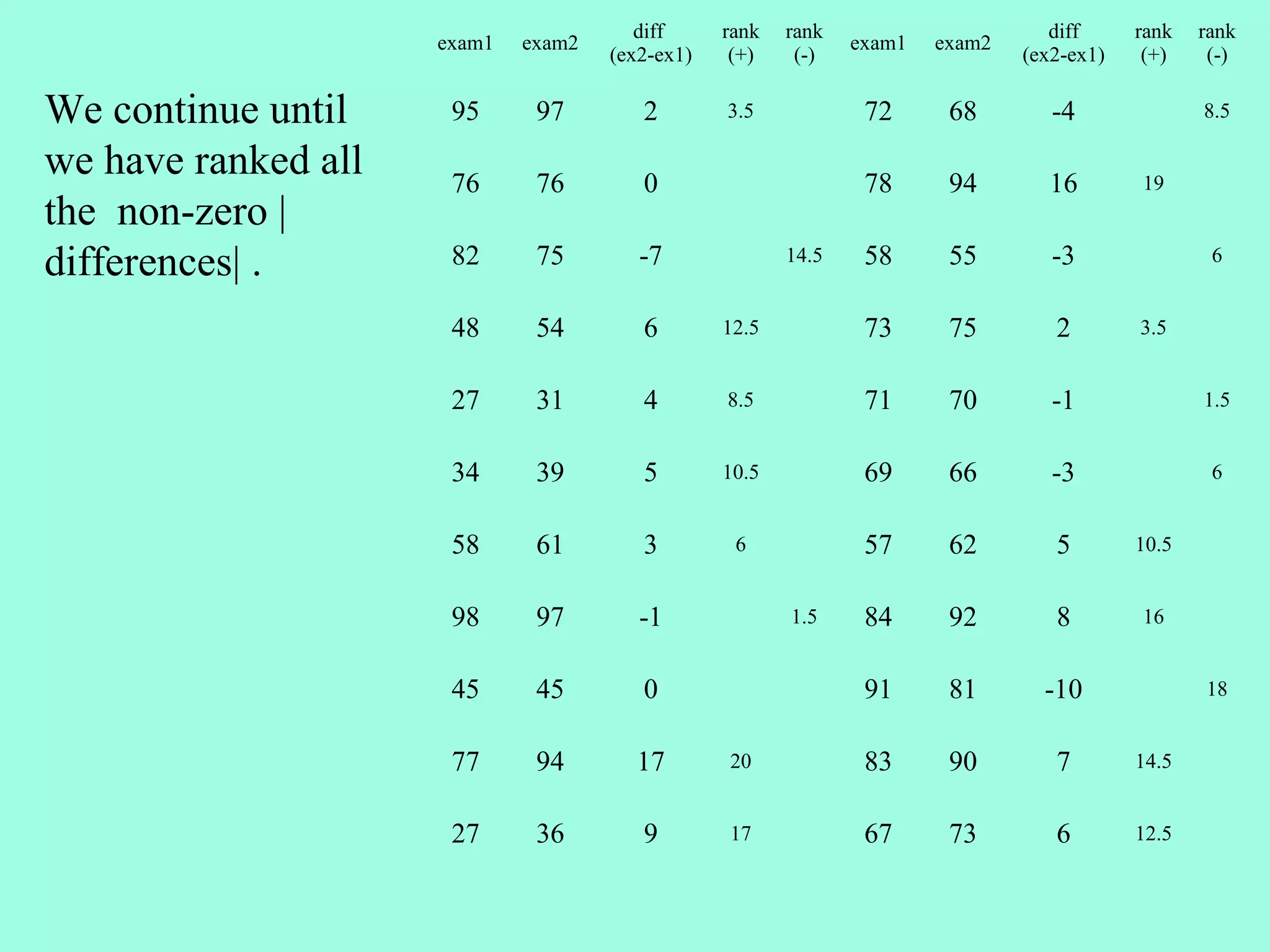
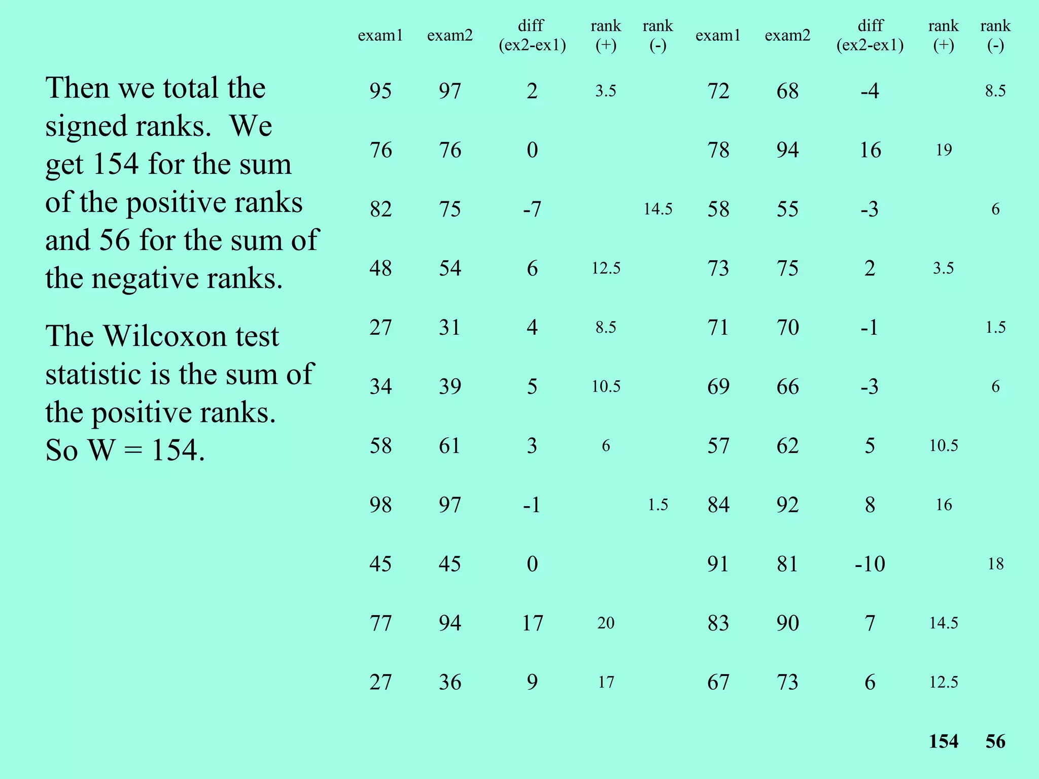
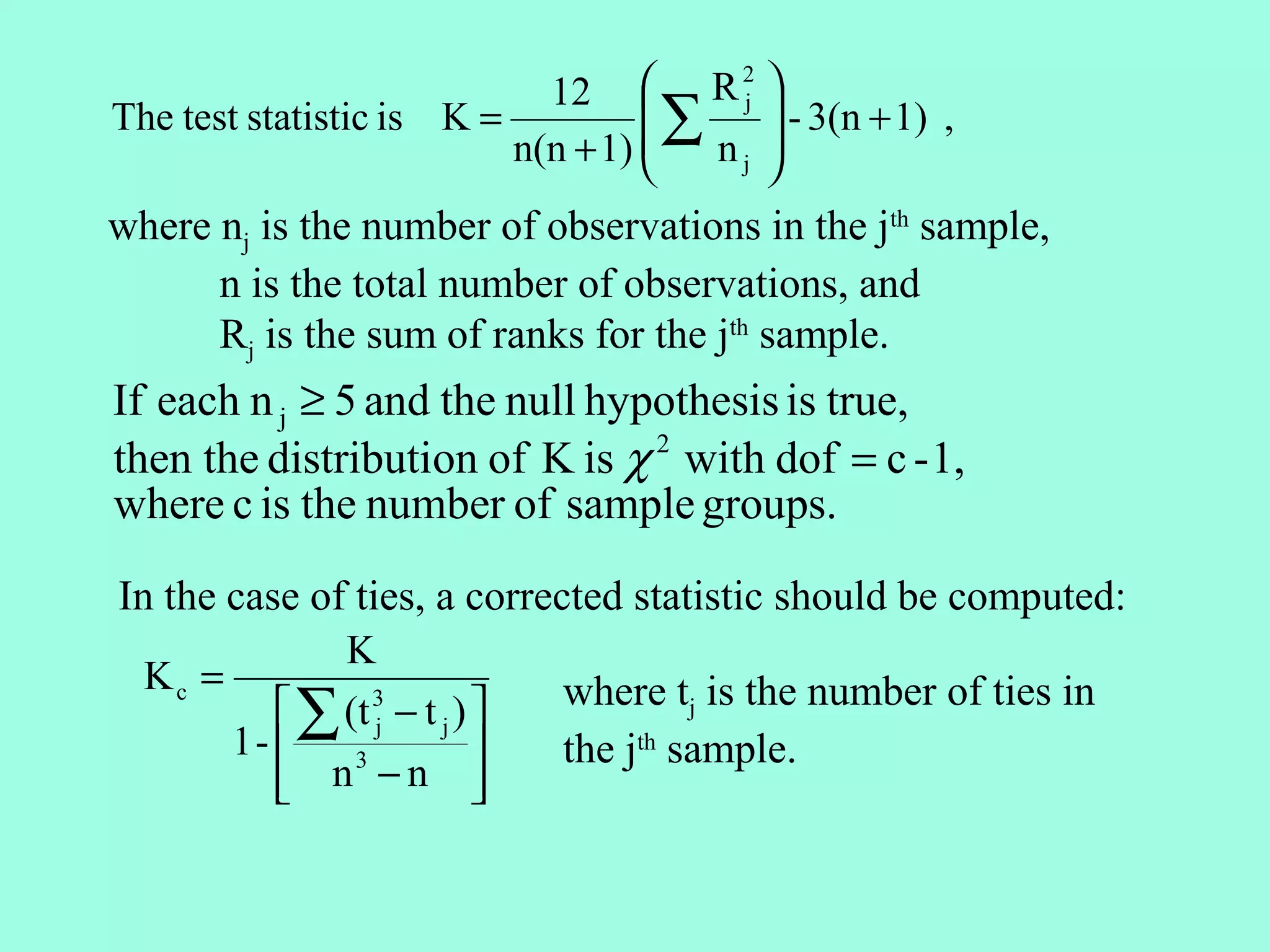
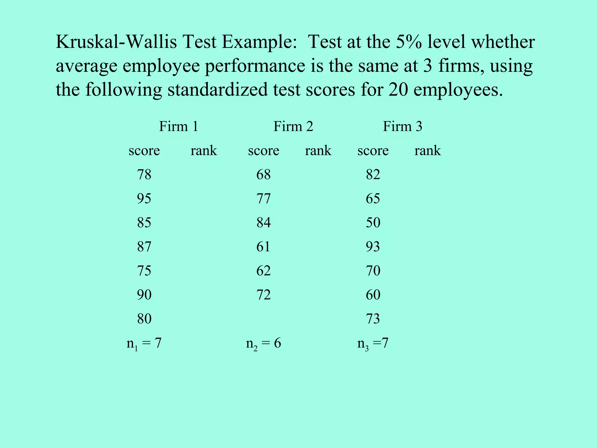
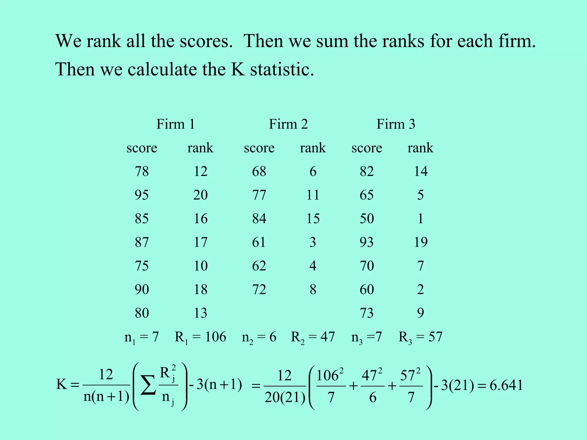
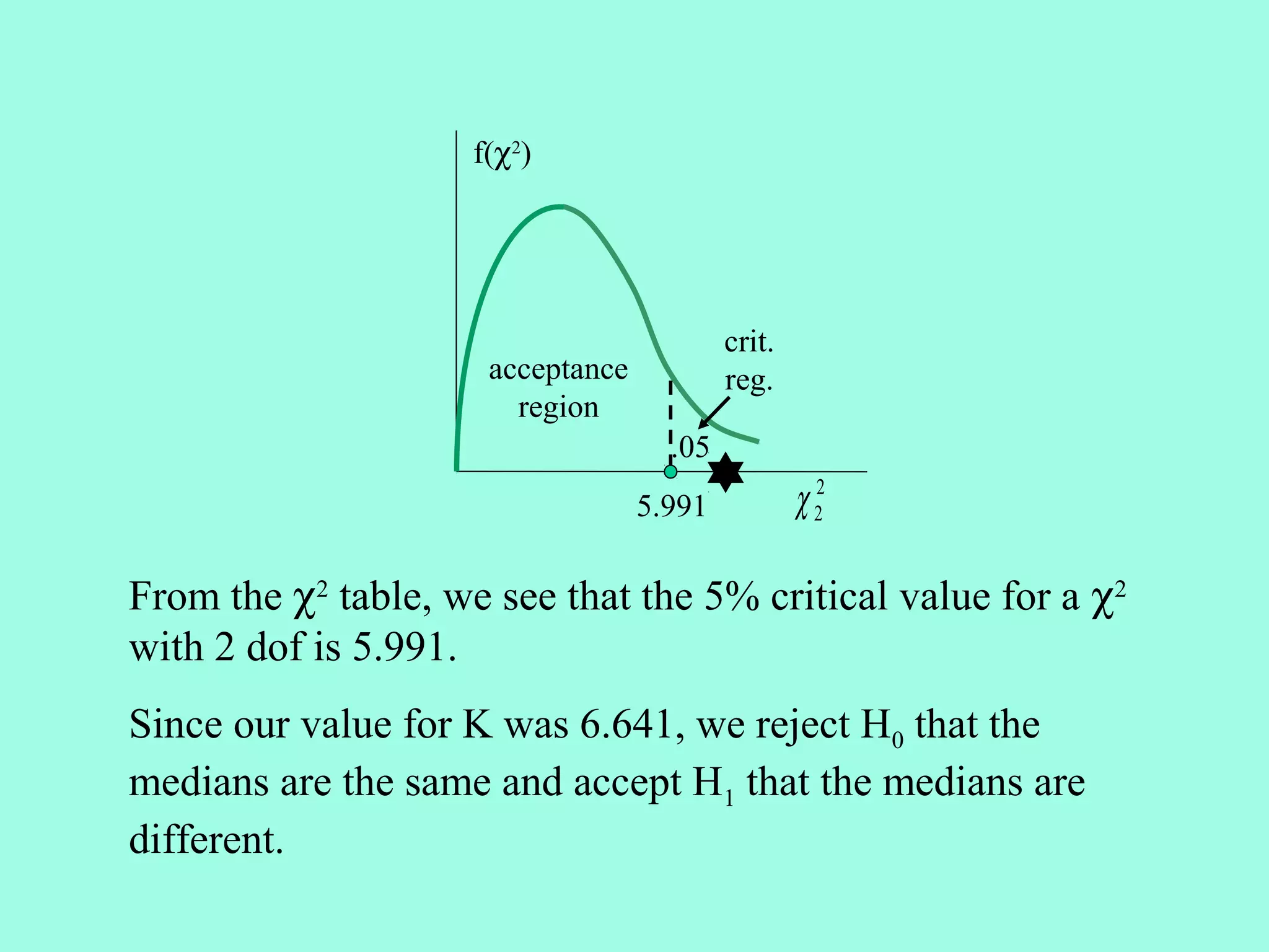
The document discusses four nonparametric statistical tests: 1. The Wilcoxon Rank Sum Test (also called the Mann-Whitney U Test) compares the medians of two independent samples and is an alternative to the independent t-test. 2. The Wilcoxon Signed Rank Test compares the medians of two dependent/paired samples and is an alternative to the paired t-test. It calculates the differences between pairs, ranks their absolute values, and sums the ranks of positive differences. 3. The Kruskal-Wallis Test compares more than two independent samples. 4. The Runs Test examines the randomness of a single sample by counting runs, or streaks, of

1. Nonparametric
Statistics

2. In previous testing, we assumed that our samples were drawn
from normally distributed populations.
This chapter introduces some techniques that do not make
that assumption.
These methods are called distribution-free or nonparametric
tests.
In situations where the normal assumption is appropriate,
nonparametric tests are less efficient than traditional
parametric methods.
Nonparametric tests frequently make use only of the order of
the observations and not the actual values.

3. In this section, we will discuss four nonparametric tests:
the Wilcoxon Rank Sum Test (or Mann-Whitney U test),
the Wilcoxon Signed Ranks Test,
the Kruskal-Wallis Test, and
the one sample test of runs.

4. The Wilcoxon Rank Sum Test
or Mann-Whitney U Test
This test is used to test whether 2 independent samples have
been drawn from populations with the same median.
It is a nonparametric substitute for the t-test on the difference
between two means.

5. Wilcoxon Rank Sum Test Example:
university Based on the following samples from
A B two universities, test at the 10% level
50 70 whether graduates from the two
52 73 schools have the same average grade
56 77 on an aptitude test.
60 80
64 83
68 85
71 87
74 88
89 96
95 99

6. First merge and rank the grades. rank grade university
Sum the ranks for each sample. 1 50 A
rank sum for university A: 74 2 52 A
rank sum for university B: 136 3 56 A
4 60 A
university 5 64 A
6 68 A Note: If there are
A B
7 70 B ties, each value
50 70 8 71 A gets the average
52 73 9 73 B rank. For example,
10 74 A if 2 values tie for
56 77
11 77 B 3th and 4th place,
60 80 both are ranked
12 80 B
64 83 13 83 B
3.5. If three
differences would
68 85 14 85 B
15 87 B
be ranked 7, 8, and
71 87 9, rank them all 8.
16 88 B
74 88 17 89 A
89 96 18 95 A
19 96 B
95 99
20 99 B

7. Here, the group from university A is considered the 1st sample.
When the samples differ in size, designate the smaller of the
2 samples as the 1st sample.
Define T1 = sum of the ranks for 1st sample .
n1 (n1 + n2 + 1)
The mean of T1 is µT1 = ,
2
n1n 2 (n1 + n2 + 1)
and the standard deviation is σ T1 = .
12
If n1 and n 2 are each at least 10, T1 is approximately normal.
T1 - µT1
So, Z = has a standard normal distribution.
σ T1
(For small sample sizes, the Z approximation is sometimes used as well.)

8. For our example, T1 = 74.
n1 (n + 1) 10(20 + 1)
µT1 = = = 105
2 2
n1n 2 (n + 1) (10)(10)(20 + 1)
σ T1 = = = 13.229
12 12
T1 - µT1 74 - 105
Z = = = -2.343.
σ T1 13.229
Since the critical values for a
2-tailed Z test at the 10%
level are 1.645 and -1.645, we critical critical
region region
reject H0 that the medians are .45 .45
the same and accept H1 that .05 .05
the medians are different. -1.645 0 1.645 Z

9. For small sample sizes, you can use Table E.8 in
your textbook, which provides the lower and upper
critical values for the Wilcoxon Rank Sum Test.
That table shows that for our 10% 2-tailed test, the
lower critical value is 82 and the upper critical value
is 128.
Since our smaller sample’s rank sum is 74, which is
outside the interval (82, 128) indicated in the table,
we reject the null hypothesis that the medians are
the same and conclude that they are different.
Equivalently, since the larger sample’s rank sum is
136, which is also outside the interval (82, 128), we
again reject the null hypothesis that the medians are
the same and conclude that they are different.

10. The Wilcoxon Signed Rank Test
This test is used to test whether 2 dependent samples have
been drawn from populations with the same median.
It is a nonparametric substitute for the paired t-test on the
difference between two means.

11. Wilcoxon Signed Rank Test Procedure
1. Calculate the differences in the paired values (Di=X1i – X2i)
2. Take absolute values of the differences and rank them (Discard
all differences that equal 0.)
3. Assign ranks Ri with the smallest rank equal to 1.
As in the rank sum test, if two or more of the differences are
equal, each difference gets the average rank. (That is, if two
differences would be ranked 3 and 4, rank them both 3.5. If
three differences would be ranked 7, 8, and 9, rank them all 8.)
4. Assign the symbol + to positive differences and – to negative
differences.
5. Calculate the Wilcoxon statistic W as the sum of the positive
ranks. So,
W= ∑ Ri+

12. Wilcoxon Signed Rank Test Procedure (cont’d)
In the following, n refers to the number of non - zero differences.
n(n + 1)
The mean of the Wilcoxon statistic W is µW =
4
The standard deviation of the Wilcoxon statistic W is
n(n + 1)(2n + 1)
σW =
24
If n is at least 20, the test statistic W is approximately normal. So we have :
W − µW
Z=
σW
(For small sample sizes, the Z approximation is sometimes used as well.)

13. diff rank rank diff rank rank
exam1 exam2 exam1 exam2
(ex2-ex1) (+) (-) (ex2-ex1) (+) (-)
Example 95 97 72 68
Suppose we have 76 76 78 94
a class with 22 82 75 58 55
students, each of
whom has two 48 54 73 75
exam grades. 27 31 71 70
We want to test at 34 39 69 66
the 5% level
58 61 57 62
whether there is a
difference in the 98 97 84 92
median grade for 45 45 91 81
the two exams.
77 94 83 90
27 36 67 73

14. diff rank rank diff rank rank
exam1 exam2 exam1 exam2
(ex2-ex1) (+) (-) (ex2-ex1) (+) (-)
We calculate the 95 97 2 72 68 -4
difference between the
exam grades: 76 76 0 78 94 16
diff = exam2 – exam 1.
82 75 -7 58 55 -3
48 54 6 73 75 2
27 31 4 71 70 -1
34 39 5 69 66 -3
58 61 3 57 62 5
98 97 -1 84 92 8
45 45 0 91 81 -10
77 94 17 83 90 7
27 36 9 67 73 6

15. diff rank rank diff rank rank
exam1 exam2 exam1 exam2
Then we rank the (ex2-ex1) (+) (-) (ex2-ex1) (+) (-)
absolute values of the 95 97 2 72 68 -4
differences from
smallest to largest, 76 76 0 78 94 16
omitting the two zero 82 75 -7 58 55 -3
differences.
48 54 6 73 75 2
The smallest non-zero
|differences| are the 27 31 4 71 70 -1 1.5
two |-1|’s. Since they 34 39 5 69 66 -3
are tied for ranks 1
and 2, we rank them 58 61 3 57 62 5
both 1.5.
98 97 -1 1.5 84 92 8
Since the differences
45 45 0 91 81 -10
were negative, we put
the ranks in the 77 94 17 83 90 7
negative column.
27 36 9 67 73 6

16. diff rank rank diff rank rank
exam1 exam2 exam1 exam2
(ex2-ex1) (+) (-) (ex2-ex1) (+) (-)
The next smallest 95 97 2 3.5 72 68 -4
non-zero |differences|
76 76 0 78 94 16
are the two |2|’s.
Since they are tied for 82 75 -7 58 55 -3
ranks 3 and 4, we
48 54 6 73 75 2 3.5
rank them both 3.5.
Since the differences 27 31 4 71 70 -1 1.5
were positive, we put 34 39 5 69 66 -3
the ranks in the
positive column. 58 61 3 57 62 5
98 97 -1 1.5 84 92 8
45 45 0 91 81 -10
77 94 17 83 90 7
27 36 9 67 73 6

17. diff rank rank diff rank rank
exam1 exam2 exam1 exam2
(ex2-ex1) (+) (-) (ex2-ex1) (+) (-)
The next smallest 95 97 2 3.5 72 68 -4
non-zero |differences| 76 76 0 78 94 16
are the two |-3|’s and
the |3|. Since they are 82 75 -7 58 55 -3 6
tied for ranks 5, 6, 48 54 6 73 75 2 3.5
and 7, we rank them
27 31 4 71 70 -1 1.5
all 6.
34 39 5 69 66 -3 6
Then we put the ranks
in the appropriately 58 61 3 6 57 62 5
signed columns. 98 97 -1 1.5 84 92 8
45 45 0 91 81 -10
77 94 17 83 90 7
27 36 9 67 73 6

18. diff rank rank diff rank rank
exam1 exam2 exam1 exam2
(ex2-ex1) (+) (-) (ex2-ex1) (+) (-)
We continue until 95 97 2 3.5 72 68 -4 8.5
we have ranked all 76 76 0 78 94 16 19
the non-zero |
differences| . 82 75 -7 14.5 58 55 -3 6
48 54 6 12.5 73 75 2 3.5
27 31 4 8.5 71 70 -1 1.5
34 39 5 10.5 69 66 -3 6
58 61 3 6 57 62 5 10.5
98 97 -1 1.5 84 92 8 16
45 45 0 91 81 -10 18
77 94 17 20 83 90 7 14.5
27 36 9 17 67 73 6 12.5

19. diff rank rank diff rank rank
exam1 exam2 exam1 exam2
(ex2-ex1) (+) (-) (ex2-ex1) (+) (-)
Then we total the 95 97 2 3.5 72 68 -4 8.5
signed ranks. We
76 76 0 78 94 16 19
get 154 for the sum
of the positive ranks 82 75 -7 14.5 58 55 -3 6
and 56 for the sum of
48 54 6 12.5 73 75 2 3.5
the negative ranks.
The Wilcoxon test 27 31 4 8.5 71 70 -1 1.5
statistic is the sum of 34 39 5 10.5 69 66 -3 6
the positive ranks.
So W = 154. 58 61 3 6 57 62 5 10.5
98 97 -1 1.5 84 92 8 16
45 45 0 91 81 -10 18
77 94 17 20 83 90 7 14.5
27 36 9 17 67 73 6 12.5
154 56

20. Since we had 22 students and 2 zero differences, the number of
non-zero differences n = 20.
n(n + 1) (20)(21)
Recall that the mean of W is µW = = = 105
4 4
The standard deviation of W is
n(n + 1)(2n + 1) 20(21)(41)
σW = = = 26.786
24 24
W − µW 154 − 105
So we have : Z= = = 1.829
σW 26.786
Since the critical values for a
2-tailed Z test at the 5% level
critical critical
are 1.96 and -1.96, we can not region
.475 .475 region
reject the null hypothesis H0 and
.025 .025
so we conclude that the medians
are the same. -1.96 0 1.96 Z

21. For small sample sizes, you can use Table E.9 in
your textbook, which provides the lower and upper
critical values for the Wilcoxon Signed Rank Test.
That table shows that for our 5% 2-tailed test, the
lower critical value is 52 and the upper critical
value is 158.
Since the sum of our positive ranks is 154, which is
inside the interval (52, 158) indicated in the table,
we can not reject the null hypothesis and so we
conclude that the medians are the same.

22. The Kruskal-Wallis Test
This test is used to test whether several populations have the
same median.
It is a nonparametric substitute for a one-factor ANOVA F-test.

23. 12  R j 
2
The test statistic is K = ∑  - 3(n + 1) ,
n(n + 1) 
 nj 

where nj is the number of observations in the jth sample,
n is the total number of observations, and
Rj is the sum of ranks for the jth sample.
If each n j ≥ 5 and the null hypothesis is true,
then the distribution of K is χ 2 with dof = c - 1,
where c is the number of sample groups.
In the case of ties, a corrected statistic should be computed:
K
Kc = where tj is the number of ties in
 ∑ (t 3 − t j ) 
j
1-   the jth sample.
 n −n 
3
 

24. Kruskal-Wallis Test Example: Test at the 5% level whether
average employee performance is the same at 3 firms, using
the following standardized test scores for 20 employees.
Firm 1 Firm 2 Firm 3
score rank score rank score rank
78 68 82
95 77 65
85 84 50
87 61 93
75 62 70
90 72 60
80 73
n1 = 7 n2 = 6 n3 =7

25. We rank all the scores. Then we sum the ranks for each firm.
Then we calculate the K statistic.
Firm 1 Firm 2 Firm 3
score rank score rank score rank
78 12 68 6 82 14
95 20 77 11 65 5
85 16 84 15 50 1
87 17 61 3 93 19
75 10 62 4 70 7
90 18 72 8 60 2
80 13 73 9
n1 = 7 R1 = 106 n2 = 6 R2 = 47 n3 =7 R3 = 57
12  R j 
2
∑  - 3(n + 1) = 12  106 2 47 2 57 2 
K= 
 7 + 6 + 7  - 3(21) = 6.641


n(n + 1)  
nj  20(21)  

26. f(χ2)
crit.
acceptance reg.
region
.05
5.991 χ 22
From the χ2 table, we see that the 5% critical value for a χ2
with 2 dof is 5.991.
Since our value for K was 6.641, we reject H0 that the
medians are the same and accept H1 that the medians are
different.

27. One sample test of runs
a test for randomness of order of occurrence

28. A run is a sequence of identical occurrences
that are followed and preceded by different
occurrences.
Example: The list of X’s & O’s below consists of 7 runs.
xxxooooxxooooxxxxoox

29. Suppose r is the number of runs, n1 is the number of
type 1 occurrences and n2 is the number of type 2
occurrences.
The mean number of runs is
2n1n 2
μr = + 1.
n1 + n 2
The standard deviation of the number of runs is
2n1n 2 (2n1n 2 - n1 - n 2 )
σr = .
(n1 + n 2 ) (n1 + n 2 − 1)
2

30. If n1 and n2 are each at least 10, then r is
approximately normal.
r - µr
So, Z=
σr
is a standard normal variable.

31. Example: A stock exhibits the following price increase (+)
and decrease (−) behavior over 25 business days. Test at the
1% whether the pattern is random.
r =16,
+ + + − − + − − − + + − + − + − − + + − + + − + − n1 (+) = 13,
2n1n 2 n2 (−) =
2(13)(12)
μr = +1 = + 1 = 13.48 12
n1 + n 2 13 + 12
2n1n 2 (2n1n 2 - n1 - n 2 ) 2(13)(12) [(2(13)(12) - 13 - 12]
σr = = = 2.44
(n1 + n 2 ) (n1 + n 2 − 1)
2
(13 + 12) (13 + 12 − 1)
2
r - µ r 16 - 13.48
Z= = = 1.03 critical critical
σr 2.44 region .495 .495
acceptance
region
.005
.005
Since the critical values for a 2-tailed 1% region
test are 2.575 and -2.575, we accept H0 -2.575 0 2.575 Z
that the pattern is random.