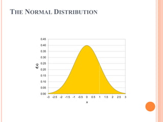
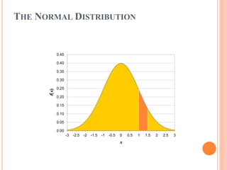
The document summarizes key concepts relating to three probability distributions: 1) The normal distribution describes variables that arise from the addition of small random effects and approximates the binomial distribution for large numbers of trials. It is used to model natural phenomena influenced by many independent factors. 2) The binomial distribution describes discrete random variables resulting from Bernoulli trials with a fixed probability of success. It gives the probability of a given number of successes in fixed number of trials. 3) The Poisson distribution approximates the binomial when the probability of success is very small but the number of trials is large. It is used to model rare random events occurring independently over an interval of time or space.

1. GUJARAT TECHNOLOGICAL UNIVERSITY
Chandkheda, Ahmadabad Afflicted
Sarvajanik college of Engineering & Technology
A
PowerPoint presentation
On
The Binomial, Poisson, and Normal Distributions.
Under subject of SQC
B.E.II, Semester- IV
(Textile Technology)
Submitted by
Group:
Submitted By:
Parth Khachariya 130420129017
Parth Chaklashiya 130420129006
---Faculty Guide---
Mr.Hiren Amin

2. THE NORMAL DISTRIBUTION
 Discovered in 1733 by de Moivre as an approximation to
the binomial distribution when the number of trails is
large
 Derived in 1809 by Gauss
 Importance lies in the Central Limit Theorem, which
states that the sum of a large number of independent
random variables (binomial, Poisson, etc.) will
approximate a normal distribution
 Example: Human height is determined by a large
number of factors, both genetic and environmental,
which are additive in their effects. Thus, it follows a
normal distribution.
Karl F. Gauss
(1777-1855)
Abraham de
Moivre (1667-
1754)

3. THE NORMAL DISTRIBUTION
 A continuous random variable is said to be normally distributed
with mean  and variance 2 if its probability density function
is
 f(x) is not the same as P(x)
 P(x) would be 0 for every x because the normal distribution
is continuous
 However, P(x1 < X ≤ x2) = f(x)dx
f (x) =
1
2
(x  )2/22
e
x1
x2

4. THE NORMAL DISTRIBUTION
0.00
0.05
0.10
0.15
0.20
0.25
0.30
0.35
0.40
0.45
-3 -2.5 -2 -1.5 -1 -0.5 0 0.5 1 1.5 2 2.5 3
f(x)
x

5. THE NORMAL DISTRIBUTION
0.00
0.05
0.10
0.15
0.20
0.25
0.30
0.35
0.40
0.45
-3 -2.5 -2 -1.5 -1 -0.5 0 0.5 1 1.5 2 2.5 3
f(x)
x

6. THE NORMAL DISTRIBUTION
LENGTH OF FISH
 A sample of rock cod in Monterey Bay suggests that the mean
length of these fish is  = 30 in. and 2 = 4 in.
 Assume that the length of rock cod is a normal random variable
 If we catch one of these fish in Monterey Bay,
 What is the probability that it will be at least 31 in. long?
 That it will be no more than 32 in. long?
 That its length will be between 26 and 29 inches?

7. THE NORMAL DISTRIBUTION
LENGTH OF FISH
 What is the probability that it will be at least 31 in. long?
0.00
0.05
0.10
0.15
0.20
0.25
25 26 27 28 29 30 31 32 33 34 35
Fish length (in.)

8. THE NORMAL DISTRIBUTION
LENGTH OF FISH
 That it will be no more than 32 in. long?
0.00
0.05
0.10
0.15
0.20
0.25
25 26 27 28 29 30 31 32 33 34 35
Fish length (in.)

9. THE NORMAL DISTRIBUTION
LENGTH OF FISH
 That its length will be between 26 and 29 inches?
0.00
0.05
0.10
0.15
0.20
0.25
25 26 27 28 29 30 31 32 33 34 35
Fish length (in.)

10. THE BINOMIAL DISTRIBUTION
BERNOULLI RANDOM VARIABLES
 Imagine a simple trial with only two possible outcomes
 Success (S)
 Failure (F)
 Examples
 Toss of a coin (heads or tails)
 Sex of a newborn (male or female)
 Survival of an organism in a region (live or die)
Jacob Bernoulli (1654-
1705)

11. THE BINOMIAL DISTRIBUTION
OVERVIEW
 Suppose that the probability of success is p
 What is the probability of failure?
 q = 1 – p
 Examples
 Toss of a coin (S = head): p = 0.5  q = 0.5
 Roll of a die (S = 1): p = 0.1667  q = 0.8333
 Fertility of a chicken egg (S = fertile): p = 0.8  q = 0.2

12. THE BINOMIAL DISTRIBUTION
OVERVIEW
 What is the probability of obtaining x successes in n trials?
 Example
 What is the probability of obtaining 2 heads from a coin that
was tossed 5 times?
P(HHTTT) = (1/2)5 = 1/32

13. THE POISSON DISTRIBUTION
OVERVIEW
 When there is a large number of
trials, but a small probability of
success, binomial calculation
becomes impractical
 Example: Number of deaths from
horse kicks in the Army in
different years
 The mean number of successes from
n trials is µ = np
 Example: 64 deaths in 20 years
from thousands of soldiers
Simeon D. Poisson (1781-
1840)

14. THE POISSON DISTRIBUTION
 If we substitute µ/n for p, and let n tend to infinity, the
binomial distribution becomes the Poisson distribution:
P(x) =
e -µµx
x!
 Poisson distribution is applied where random events in space or
time are expected to occur
 Deviation from Poisson distribution may indicate some degree
of non-randomness in the events under study
 Investigation of cause may be of interest

15. THE POISSON DISTRIBUTION
EMISSION OF -PARTICLES
 Rutherford, Geiger, and Bateman (1910) counted the
number of -particles emitted by a film of polonium in
2608 successive intervals of one-eighth of a minute
 What is n?
 What is p?
 Do their data follow a Poisson distribution?

16. THE POISSON DISTRIBUTION
EMISSION OF -PARTICLES
No. -particles Observed
0 57
1 203
2 383
3 525
4 532
5 408
6 273
7 139
8 45
9 27
10 10
11 4
12 0
13 1
14 1
Over 14 0
Total 2608
 Calculation of µ:
µ = No. of particles per interval
= 10097/2608
= 3.87
 Expected values:
2680  P(x) =
e -3.87(3.87)x
x!
2608 

17. THE POISSON DISTRIBUTION
EMISSION OF -PARTICLES
No. -particles Observed Expected
0 57 54
1 203 210
2 383 407
3 525 525
4 532 508
5 408 394
6 273 254
7 139 140
8 45 68
9 27 29
10 10 11
11 4 4
12 0 1
13 1 1
14 1 1
Over 14 0 0
Total 2608 2680

18. THE POISSON DISTRIBUTION
EMISSION OF -PARTICLES
Random events
Regular events
Clumped events