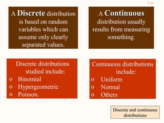
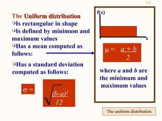
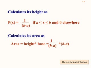
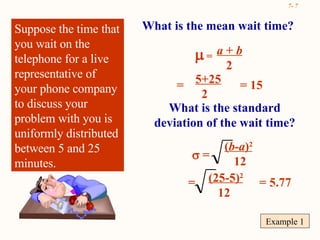
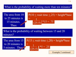
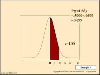
Chapter Seven McGraw-Hill/Irwin © 2005 The McGraw-Hill Companies, Inc., All Rights Reserved.
Goals Chapter Seven Continuous Probability Distributions GOALS When you have completed this chapter, you will be able to: ONE Understand the difference between discrete and continuous distributions . TWO Compute the mean and the standard deviation for a uniform distribution. THREE Compute probabilities using the uniform distribution. FOUR List the characteristics of the normal probability distribution.
Goals Chapter Seven  continued GOALS When you have completed this chapter, you will be able to: FIVE   Define and calculate  z  values. SIX Determine the probability an observation will lie between two points using the standard normal distribution.  SEVEN Determine the probability an observation will be above or below a given value using the standard normal distribution. EIGHT Use the normal distribution to approximate the binomial probability distribution. Continuous Probability Distributions
Discrete and continuous distributions A  Discrete   distribution is based on random variables which can assume only clearly separated values. Discrete distributions studied include:  Binomial  Hypergeometric Poisson. A  Continuous  distribution usually results from measuring something. Continuous distributions include:  Uniform  Normal  Others
The uniform distribution The  Uniform distribution   Is rectangular in shape Is defined by minimum and maximum values Has a mean computed as follows: a + b   2   = where  a  and  b  are the minimum and maximum values Has a standard deviation computed as follows:    = (b-a) 2 12 f(x) x
The uniform distribution Calculates its height as P(x) =  if  a   <  x  <   b  and 0 elsewhere 1 ( b-a ) Calculates its area as Area = height* base =  *( b-a )   1 ( b-a )
Example 1 Suppose the time that you wait on the telephone for a live representative of your phone company to discuss your problem with you is uniformly distributed between 5 and 25 minutes. What is the mean wait time? a  +  b   2    = = 5+25 2 = 15 What is the standard deviation of the wait time?    = ( b-a ) 2 12 = (25-5) 2 12 = 5.77
Example 2 continued What is the probability of waiting more than ten minutes? The area from 10 to 25 minutes is 15 minutes.  Thus: P(10  <  wait time  <  25) = height*base  =  1 (25-5) *15 = .75 What is the probability of waiting between 15 and 20 minutes? The area from 15 to 20 minutes is 5 minutes.  Thus: P(15  <  wait time  <  20) = height*base  =  1 (25-5) *5 = .25
is  bell-shaped  and has a single peak at the center of the distribution.  Is  symmetrical  about the mean. is  asymptotic .  That is the curve gets closer and closer to the  X -axis but never actually touches it. Has its  mean,   , to determine its location and its  standard deviation,   , to determine its dispersion. The  Normal  probability distribution
Characteristics of a Normal Distribution Mean, median, and mode are equal Theoretically, curve extends to infinity a Normal curve is symmetrical - 5 0 . 4 0 . 3 0 . 2 0 . 1 . 0 x f ( x r a l i t r b u i o n :  = 0 ,   = 1
The Standard Normal  Probability Distribution A  z- value   is the distance between a selected value, designated  X , and the population mean   , divided by the population standard deviation,   .  The formula is: It is also called the  z  distribution. The  standard normal  distribution is a normal distribution with a mean of 0 and a standard deviation of 1.
Example 2 = $2,200 - $2000 $200 = 1.00 The bi-monthly starting salaries of recent MBA graduates follows the normal distribution with a mean of $2,000 and a standard deviation of $200.  What is the  z- value  for a salary of $2,200?
EXAMPLE 2  continued What is the z-value for $1,700? A  z-v alue  of 1 indicates that the value of $2,200 is one standard deviation above the mean of $2,000. A  z-v alue  of –1.50 indicates that $1,700 is 1.5 standard deviation below the mean of $2000.
Areas Under the Normal Curve Practically all is within three standard deviations of the mean.     +  3  About 68 percent of the area under the normal curve is within one standard deviation of the mean.    +  1  About 95 percent is within two standard deviations of the mean.     +  2 
Example 3 The daily water usage per person in New Providence, New Jersey is normally distributed with a mean of 20 gallons and a standard deviation of 5 gallons.  About 68 percent of those living in New Providence will use how many gallons of water?  About 68% of the daily water usage will lie between 15 and 25 gallons ( +  1   ).
EXAMPLE 4 What is the probability that a person from New Providence selected at random will use between 20 and 24 gallons per day?
Example 4  continued The area under a normal curve between a  z -value of 0 and a  z -value of 0.80 is 0.2881.  We conclude that 28.81 percent of the residents use between 20 and 24 gallons of water per day. See the following diagram
 
EXAMPLE 4   continued What percent of the population use between 18 and 26 gallons per day?
EXAMPLE 4  continued We conclude that 54.03 percent of the residents use between 18 and 26 gallons of water per day. The area associated with a  z- value of –0.40 is .1554. The area associated with a  z -value of 1.20 is  .3849. Adding these areas, the result is .5403.
EXAMPLE 5 Professor Mann has determined that the scores  in his statistics course are approximately normally distributed with a mean of 72 and a standard deviation of 5.  He announces to the class that the top 15 percent of the scores will earn an A.  What is the lowest score a student can earn and still receive an A?
EXAMPLE 5  continued The  z -value associated corresponding to 35 percent is about 1.04. To begin let  X  be the score that separates an  A  from a  B.  If 15 percent of the students score more than  X,  then 35 percent must score between the mean of 72 and  X.
EXAMPLE 5  continued Those with a score of 77.2 or more earn an  A. We let  z  equal 1.04 and solve the standard normal equation for  X.  T he result is the score that separates students that earned an  A  from those that earned a  B.
The Normal Approximation to the Binomial The normal probability distribution is generally a good approximation to the binomial probability distribution when  n    and  n(1-    )  are both greater than 5. The normal distribution (a continuous distribution) yields a good approximation of the binomial distribution (a discrete distribution) for large values of  n.
The Normal Approximation  continued Recall for the binomial experiment: There are only two mutually exclusive outcomes (success or failure) on each trial. A binomial distribution results from counting the number of successes. Each trial is independent.   The probability  is fixed from trial to trial, and the number of trials  n  is also fixed.
Continuity Correction Factor The value .5 subtracted or added, depending on the problem, to a selected value when a binomial probability distribution (a discrete probability distribution) is being approximated by a continuous probability distribution (the normal distribution). Continuity Correction Factor
Continuity Correction Factor For the probability that  fewer than X  occur, use the area below (X-.5). How to Apply the Correction Factor: For the probability  at least   X  occur, use the area above (X-.5). For the probability that  more than   X  occur, use the area above (X+.5). For the probability that  X or fewer  occur, use the area below (X+.5).
EXAMPLE 6 A recent study by a marketing research firm showed that 15% of American households owned a video camera.  For a sample of 200 homes, how many of the homes would you expect to have video cameras?  This is the mean of a binomial distribution.
EXAMPLE 6  continued  What is the standard deviation? What is the variance?
EXAMPLE 6  continued  What is the probability that less than 40 homes in the sample have video cameras?  We use the correction factor (X-.5) for fewer than, so  X-.5  is 39.5.  The value of  z  is 1.88.
From Appendix D the area between 0 and 1.88 on the  z  scale is .4699. So the area to the left of 1.88 is .5000 + .4699 = .9699. The likelihood that less than 40 of the 200 homes have a video camera is about 97%.  EXAMPLE 6  continued
 

Chapter 7 Powerpoint

  • 1.
    Chapter Seven McGraw-Hill/Irwin© 2005 The McGraw-Hill Companies, Inc., All Rights Reserved.
  • 2.
    Goals Chapter SevenContinuous Probability Distributions GOALS When you have completed this chapter, you will be able to: ONE Understand the difference between discrete and continuous distributions . TWO Compute the mean and the standard deviation for a uniform distribution. THREE Compute probabilities using the uniform distribution. FOUR List the characteristics of the normal probability distribution.
  • 3.
    Goals Chapter Seven continued GOALS When you have completed this chapter, you will be able to: FIVE Define and calculate z values. SIX Determine the probability an observation will lie between two points using the standard normal distribution. SEVEN Determine the probability an observation will be above or below a given value using the standard normal distribution. EIGHT Use the normal distribution to approximate the binomial probability distribution. Continuous Probability Distributions
  • 4.
    Discrete and continuousdistributions A Discrete distribution is based on random variables which can assume only clearly separated values. Discrete distributions studied include: Binomial Hypergeometric Poisson. A Continuous distribution usually results from measuring something. Continuous distributions include: Uniform Normal Others
  • 5.
    The uniform distributionThe Uniform distribution Is rectangular in shape Is defined by minimum and maximum values Has a mean computed as follows: a + b 2  = where a and b are the minimum and maximum values Has a standard deviation computed as follows:  = (b-a) 2 12 f(x) x
  • 6.
    The uniform distributionCalculates its height as P(x) = if a < x < b and 0 elsewhere 1 ( b-a ) Calculates its area as Area = height* base = *( b-a ) 1 ( b-a )
  • 7.
    Example 1 Supposethe time that you wait on the telephone for a live representative of your phone company to discuss your problem with you is uniformly distributed between 5 and 25 minutes. What is the mean wait time? a + b 2   = = 5+25 2 = 15 What is the standard deviation of the wait time?  = ( b-a ) 2 12 = (25-5) 2 12 = 5.77
  • 8.
    Example 2 continuedWhat is the probability of waiting more than ten minutes? The area from 10 to 25 minutes is 15 minutes. Thus: P(10 < wait time < 25) = height*base = 1 (25-5) *15 = .75 What is the probability of waiting between 15 and 20 minutes? The area from 15 to 20 minutes is 5 minutes. Thus: P(15 < wait time < 20) = height*base = 1 (25-5) *5 = .25
  • 9.
    is bell-shaped and has a single peak at the center of the distribution. Is symmetrical about the mean. is asymptotic . That is the curve gets closer and closer to the X -axis but never actually touches it. Has its mean,  , to determine its location and its standard deviation,  , to determine its dispersion. The Normal probability distribution
  • 10.
    Characteristics of aNormal Distribution Mean, median, and mode are equal Theoretically, curve extends to infinity a Normal curve is symmetrical - 5 0 . 4 0 . 3 0 . 2 0 . 1 . 0 x f ( x r a l i t r b u i o n :  = 0 ,   = 1
  • 11.
    The Standard Normal Probability Distribution A z- value is the distance between a selected value, designated X , and the population mean  , divided by the population standard deviation,  . The formula is: It is also called the z distribution. The standard normal distribution is a normal distribution with a mean of 0 and a standard deviation of 1.
  • 12.
    Example 2 =$2,200 - $2000 $200 = 1.00 The bi-monthly starting salaries of recent MBA graduates follows the normal distribution with a mean of $2,000 and a standard deviation of $200. What is the z- value for a salary of $2,200?
  • 13.
    EXAMPLE 2 continued What is the z-value for $1,700? A z-v alue of 1 indicates that the value of $2,200 is one standard deviation above the mean of $2,000. A z-v alue of –1.50 indicates that $1,700 is 1.5 standard deviation below the mean of $2000.
  • 14.
    Areas Under theNormal Curve Practically all is within three standard deviations of the mean.  + 3  About 68 percent of the area under the normal curve is within one standard deviation of the mean.  + 1  About 95 percent is within two standard deviations of the mean.  + 2 
  • 15.
    Example 3 Thedaily water usage per person in New Providence, New Jersey is normally distributed with a mean of 20 gallons and a standard deviation of 5 gallons. About 68 percent of those living in New Providence will use how many gallons of water? About 68% of the daily water usage will lie between 15 and 25 gallons ( + 1  ).
  • 16.
    EXAMPLE 4 Whatis the probability that a person from New Providence selected at random will use between 20 and 24 gallons per day?
  • 17.
    Example 4 continued The area under a normal curve between a z -value of 0 and a z -value of 0.80 is 0.2881. We conclude that 28.81 percent of the residents use between 20 and 24 gallons of water per day. See the following diagram
  • 18.
  • 19.
    EXAMPLE 4 continued What percent of the population use between 18 and 26 gallons per day?
  • 20.
    EXAMPLE 4 continued We conclude that 54.03 percent of the residents use between 18 and 26 gallons of water per day. The area associated with a z- value of –0.40 is .1554. The area associated with a z -value of 1.20 is .3849. Adding these areas, the result is .5403.
  • 21.
    EXAMPLE 5 ProfessorMann has determined that the scores in his statistics course are approximately normally distributed with a mean of 72 and a standard deviation of 5. He announces to the class that the top 15 percent of the scores will earn an A. What is the lowest score a student can earn and still receive an A?
  • 22.
    EXAMPLE 5 continued The z -value associated corresponding to 35 percent is about 1.04. To begin let X be the score that separates an A from a B. If 15 percent of the students score more than X, then 35 percent must score between the mean of 72 and X.
  • 23.
    EXAMPLE 5 continued Those with a score of 77.2 or more earn an A. We let z equal 1.04 and solve the standard normal equation for X. T he result is the score that separates students that earned an A from those that earned a B.
  • 24.
    The Normal Approximationto the Binomial The normal probability distribution is generally a good approximation to the binomial probability distribution when n  and n(1-  ) are both greater than 5. The normal distribution (a continuous distribution) yields a good approximation of the binomial distribution (a discrete distribution) for large values of n.
  • 25.
    The Normal Approximation continued Recall for the binomial experiment: There are only two mutually exclusive outcomes (success or failure) on each trial. A binomial distribution results from counting the number of successes. Each trial is independent. The probability is fixed from trial to trial, and the number of trials n is also fixed.
  • 26.
    Continuity Correction FactorThe value .5 subtracted or added, depending on the problem, to a selected value when a binomial probability distribution (a discrete probability distribution) is being approximated by a continuous probability distribution (the normal distribution). Continuity Correction Factor
  • 27.
    Continuity Correction FactorFor the probability that fewer than X occur, use the area below (X-.5). How to Apply the Correction Factor: For the probability at least X occur, use the area above (X-.5). For the probability that more than X occur, use the area above (X+.5). For the probability that X or fewer occur, use the area below (X+.5).
  • 28.
    EXAMPLE 6 Arecent study by a marketing research firm showed that 15% of American households owned a video camera. For a sample of 200 homes, how many of the homes would you expect to have video cameras? This is the mean of a binomial distribution.
  • 29.
    EXAMPLE 6 continued What is the standard deviation? What is the variance?
  • 30.
    EXAMPLE 6 continued What is the probability that less than 40 homes in the sample have video cameras? We use the correction factor (X-.5) for fewer than, so X-.5 is 39.5. The value of z is 1.88.
  • 31.
    From Appendix Dthe area between 0 and 1.88 on the z scale is .4699. So the area to the left of 1.88 is .5000 + .4699 = .9699. The likelihood that less than 40 of the 200 homes have a video camera is about 97%. EXAMPLE 6 continued
  • 32.