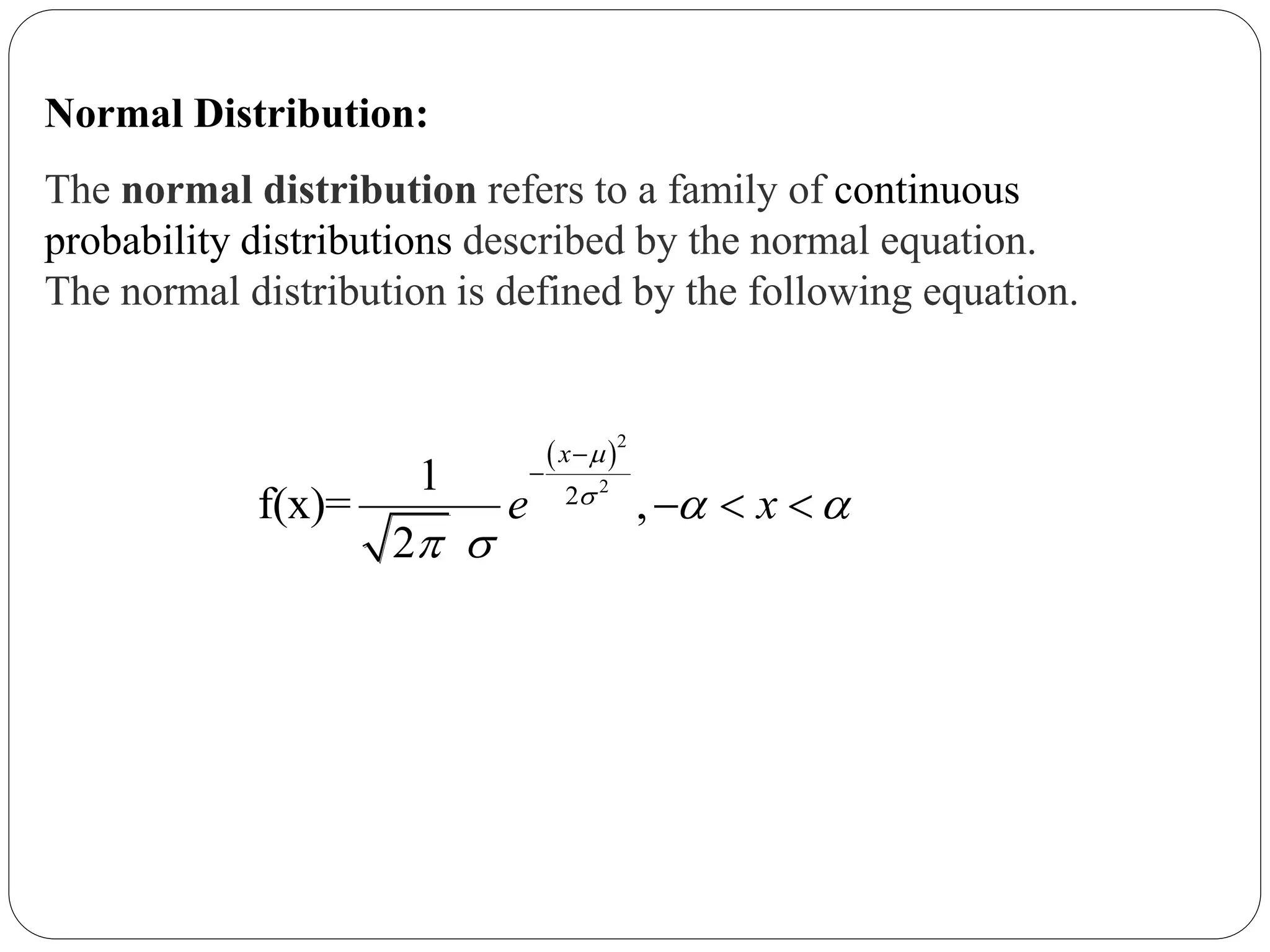
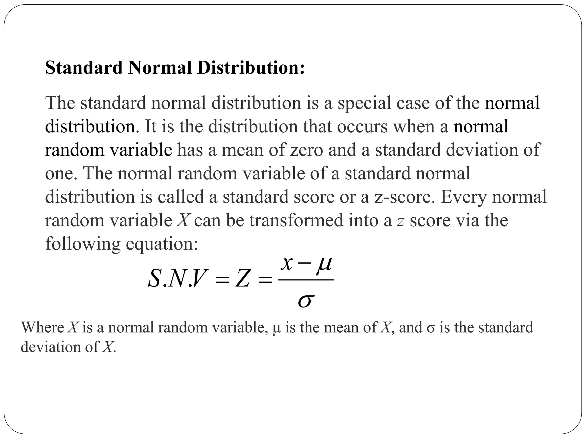
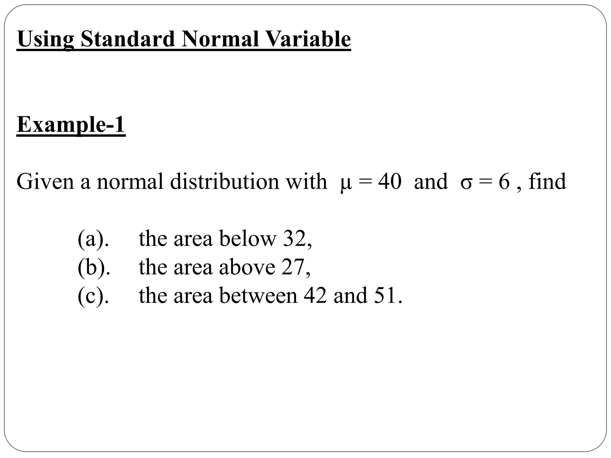
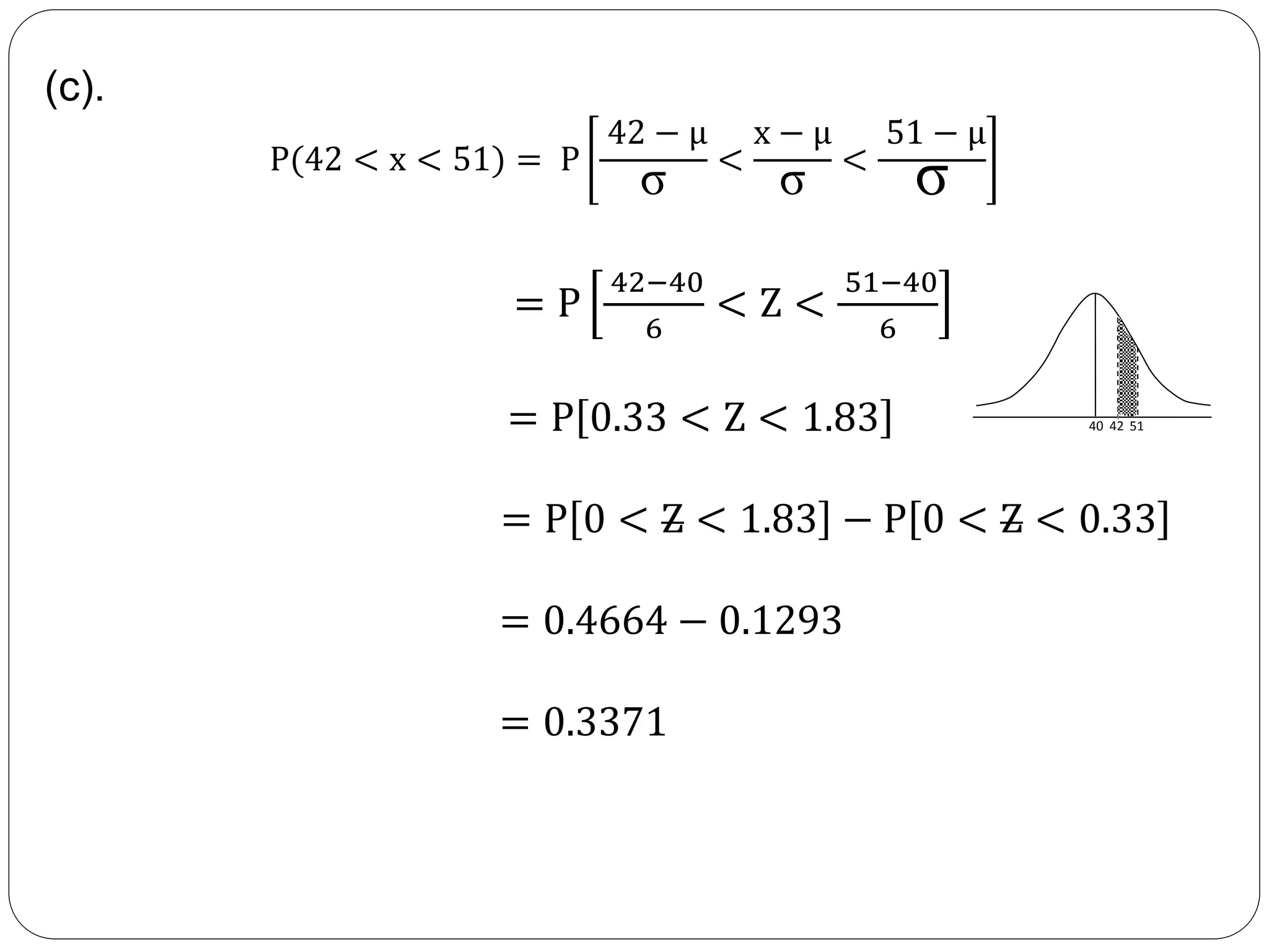
Standard Normal Distribution
NADEEM UDDIN
ASSOCIATE PROFESSOR
OF STATISTICS
A continuous random variable is a random variable where
the data can take infinite values.
For example
measuring the time taken for something to be done is
continuous random variable. A continuous random variable
can be describe by a graph and by a function.
A normal distribution, sometimes called the bell curve, The
bell curve is symmetrical. Half of the data will fall to the left
of the mean and half will fall to the right.
Normal Distribution:
The normal distribution refers to a family of continuous
probability distributions described by the normal equation.
The normal distribution is defined by the following equation.
 2
2
2
1
f(x)= ,
2
x
e x


 
 


  
Standard Normal Distribution:
The standard normal distribution is a special case of the normal
distribution. It is the distribution that occurs when a normal
random variable has a mean of zero and a standard deviation of
one. The normal random variable of a standard normal
distribution is called a standard score or a z-score. Every normal
random variable X can be transformed into a z score via the
following equation:
. .
x
S N V Z



 
Where X is a normal random variable, μ is the mean of X, and σ is the standard
deviation of X.
Using Standard Normal Variable
Example-1
Given a normal distribution with µ = 40 and σ = 6 , find
(a). the area below 32,
(b). the area above 27,
(c). the area between 42 and 51.
Solution :
Since µ = 40 and σ = 6, X ̴ N(40,62)
You need to find p(x < 32).To be able to use the standard normal
table, standardize the x variable by subtracting the mean 40 then
dividing by the standard deviation, 6.Appling this to both sides of the
inequality x<32.
(a). P x < 32 = P
x−μ
σ <
32−μ
σ
= P Z <
32−40
6
= P Z < −1.33 = 0.0918
32 40
(b). P(x > 27) = P
x−μ
σ >
27−μ
σ
= P Z >
27−40
6
= P Z > −2.17
=1 - P Z < −2.17
= 1 − 0.0150
= 0.9850
27 40
(c).
P(42 < x < 51) = P
42 − μ
σ <
x − μ
σ <
51 − μ
σ
= P
42−40
6
< Z <
51−40
6
= P 0.33 < Z < 1.83
= P 0 < Z < 1.83 − P 0 < Z < 0.33
= 0.4664 − 0.1293
= 0.3371
40 42 51
Example-2
The life of a certain make of saver bulb is known to be
normally distributed with a mean life of 2000 hours and a
standard deviation of 120 hours. In a batch of 5000 saver
bulbs, estimate the number of saver bulbs that the life of
such a bulb will be
(a)Less than 1950 hours’
(b)Greater than 2150 hours’
(c) From 1850 hours to 2090 hours.
Solution :
(a). P(x < 1950) = P
x−μ
σ <
1950−μ
σ
= P Z <
1950−2000
120
= P Z < −0.42
= 0.3372
Number of saver bulb life less than 1950 hours is ;
0.3372×5000 = 1686 bulbs.
1950 2000
(b). P(x > 2150) = P
x−μ
σ >
2150−μ
σ
= P Z >
2150−2000
120
= P Z > 1.25
=1 - P Z < 1.25
= 1 − 0.8944
= 0.1056
Number of saver bulb life greater than 2150 hours is ;
0.1056×5000 = 528 bulbs.
2000 2150
(c).
P(1850 < x < 2090) = P
1850 − μ
σ
<
x − μ
σ
<
2090 − μ
σ
= P
1850−2000
120
< Z <
2090−2000
120
= P −1.25 < Z < 0.75
= P 0 < Z < 0.75 − P −1.25 < Z < 0
= 0.7734 − 0.1056
= 0.6678
Number of saver bulb life between 1850 hours to 2090 hours is
0.6678×5000 = 3339 bulbs.
1850 2000 2090
Example-3
If X is normally distributed with parameters µ = 6 and 𝜎2 = 16 find
(a) 𝑃 𝑥 − 4 ˂ 8
(b) 𝑃( 𝑥 − 4 > 8)
(c) 𝑃( 𝑥 − 4 > 8) by using complementary law.
Solution: (a)
𝑃 𝑥 − 4 < 8 = 𝑃(−4 ˂ 𝑥˂12)
𝑃 𝑥 − 4 < 8 = 𝑃(
−4−𝜇
𝜎
˂
𝑥−𝜇
𝜎
˂
12−𝜇
𝜎
)
𝑃 𝑥 − 4 < 8 = 𝑃(
−4−6
4
˂ 𝑍 ˂
12−6
4
)
𝑃 𝑥 − 4 < 8 = 𝑃(−2.50˂ 𝑍 ˂1.50)
𝑃 𝑥 − 4 < 8 = 𝑃 𝑍 ˂ 1.50 − 𝑃 𝑍 ˂ − 2.50
𝑃 𝑥 − 4 < 8 = 0.9332 − 0.0062
𝑃 𝑥 − 4 < 8 = 0.9270
(b)
𝑃 𝑥 − 4 > 8 = 1 − 𝑃 𝑥 − 4 < 8
𝑃 𝑥 − 4 > 8 = 1 − 𝑃(−4 ˂ 𝑥˂12)
𝑃 𝑥 − 4 > 8 = 1 − 𝑃(
−4−𝜇
𝜎
˂
𝑥−𝜇
𝜎
˂
12−𝜇
𝜎
)
𝑃 𝑥 − 4 > 8 = 1 − 𝑃(
−4−6
4
˂ 𝑍 ˂
12−6
4
)
𝑃 𝑥 − 4 > 8 = 1 − 𝑃(−2.50˂ 𝑍 ˂1.50)
𝑃 𝑥 − 4 > 8 = 1 − {𝑃 𝑍 ˂ 1.50 − 𝑃 𝑍 ˂ − 2.50 }
𝑃 𝑥 − 4 > 8 = 1 − (0.9332 − 0.0062)
𝑃 𝑥 − 4 > 8 = 1 − 0.9270
𝑃 𝑥 − 4 > 8 = 0.0730
(c)
𝑃 𝑥 − 4 > 8 = 1 − 𝑃 𝑥 − 4 < 8
𝑃 𝑥 − 4 > 8 = 1 − 𝑃 −4 ˂ 𝑥˂12
𝑃 𝑥 − 4 > 8 = 1 − 0.9270 (from part a)
𝑃 𝑥 − 4 > 8 = 0.0730

Standard normal distribution

  • 1.
    Standard Normal Distribution NADEEMUDDIN ASSOCIATE PROFESSOR OF STATISTICS
  • 2.
    A continuous randomvariable is a random variable where the data can take infinite values. For example measuring the time taken for something to be done is continuous random variable. A continuous random variable can be describe by a graph and by a function. A normal distribution, sometimes called the bell curve, The bell curve is symmetrical. Half of the data will fall to the left of the mean and half will fall to the right.
  • 3.
    Normal Distribution: The normaldistribution refers to a family of continuous probability distributions described by the normal equation. The normal distribution is defined by the following equation.  2 2 2 1 f(x)= , 2 x e x           
  • 4.
    Standard Normal Distribution: Thestandard normal distribution is a special case of the normal distribution. It is the distribution that occurs when a normal random variable has a mean of zero and a standard deviation of one. The normal random variable of a standard normal distribution is called a standard score or a z-score. Every normal random variable X can be transformed into a z score via the following equation: . . x S N V Z      Where X is a normal random variable, μ is the mean of X, and σ is the standard deviation of X.
  • 6.
    Using Standard NormalVariable Example-1 Given a normal distribution with µ = 40 and σ = 6 , find (a). the area below 32, (b). the area above 27, (c). the area between 42 and 51.
  • 7.
    Solution : Since µ= 40 and σ = 6, X ̴ N(40,62) You need to find p(x < 32).To be able to use the standard normal table, standardize the x variable by subtracting the mean 40 then dividing by the standard deviation, 6.Appling this to both sides of the inequality x<32. (a). P x < 32 = P x−μ σ < 32−μ σ = P Z < 32−40 6 = P Z < −1.33 = 0.0918 32 40
  • 8.
    (b). P(x >27) = P x−μ σ > 27−μ σ = P Z > 27−40 6 = P Z > −2.17 =1 - P Z < −2.17 = 1 − 0.0150 = 0.9850 27 40
  • 9.
    (c). P(42 < x< 51) = P 42 − μ σ < x − μ σ < 51 − μ σ = P 42−40 6 < Z < 51−40 6 = P 0.33 < Z < 1.83 = P 0 < Z < 1.83 − P 0 < Z < 0.33 = 0.4664 − 0.1293 = 0.3371 40 42 51
  • 10.
    Example-2 The life ofa certain make of saver bulb is known to be normally distributed with a mean life of 2000 hours and a standard deviation of 120 hours. In a batch of 5000 saver bulbs, estimate the number of saver bulbs that the life of such a bulb will be (a)Less than 1950 hours’ (b)Greater than 2150 hours’ (c) From 1850 hours to 2090 hours.
  • 11.
    Solution : (a). P(x< 1950) = P x−μ σ < 1950−μ σ = P Z < 1950−2000 120 = P Z < −0.42 = 0.3372 Number of saver bulb life less than 1950 hours is ; 0.3372×5000 = 1686 bulbs. 1950 2000
  • 12.
    (b). P(x >2150) = P x−μ σ > 2150−μ σ = P Z > 2150−2000 120 = P Z > 1.25 =1 - P Z < 1.25 = 1 − 0.8944 = 0.1056 Number of saver bulb life greater than 2150 hours is ; 0.1056×5000 = 528 bulbs. 2000 2150
  • 13.
    (c). P(1850 < x< 2090) = P 1850 − μ σ < x − μ σ < 2090 − μ σ = P 1850−2000 120 < Z < 2090−2000 120 = P −1.25 < Z < 0.75 = P 0 < Z < 0.75 − P −1.25 < Z < 0 = 0.7734 − 0.1056 = 0.6678 Number of saver bulb life between 1850 hours to 2090 hours is 0.6678×5000 = 3339 bulbs. 1850 2000 2090
  • 14.
    Example-3 If X isnormally distributed with parameters µ = 6 and 𝜎2 = 16 find (a) 𝑃 𝑥 − 4 ˂ 8 (b) 𝑃( 𝑥 − 4 > 8) (c) 𝑃( 𝑥 − 4 > 8) by using complementary law. Solution: (a) 𝑃 𝑥 − 4 < 8 = 𝑃(−4 ˂ 𝑥˂12) 𝑃 𝑥 − 4 < 8 = 𝑃( −4−𝜇 𝜎 ˂ 𝑥−𝜇 𝜎 ˂ 12−𝜇 𝜎 ) 𝑃 𝑥 − 4 < 8 = 𝑃( −4−6 4 ˂ 𝑍 ˂ 12−6 4 ) 𝑃 𝑥 − 4 < 8 = 𝑃(−2.50˂ 𝑍 ˂1.50)
  • 15.
    𝑃 𝑥 −4 < 8 = 𝑃 𝑍 ˂ 1.50 − 𝑃 𝑍 ˂ − 2.50 𝑃 𝑥 − 4 < 8 = 0.9332 − 0.0062 𝑃 𝑥 − 4 < 8 = 0.9270 (b) 𝑃 𝑥 − 4 > 8 = 1 − 𝑃 𝑥 − 4 < 8 𝑃 𝑥 − 4 > 8 = 1 − 𝑃(−4 ˂ 𝑥˂12) 𝑃 𝑥 − 4 > 8 = 1 − 𝑃( −4−𝜇 𝜎 ˂ 𝑥−𝜇 𝜎 ˂ 12−𝜇 𝜎 ) 𝑃 𝑥 − 4 > 8 = 1 − 𝑃( −4−6 4 ˂ 𝑍 ˂ 12−6 4 ) 𝑃 𝑥 − 4 > 8 = 1 − 𝑃(−2.50˂ 𝑍 ˂1.50)
  • 16.
    𝑃 𝑥 −4 > 8 = 1 − {𝑃 𝑍 ˂ 1.50 − 𝑃 𝑍 ˂ − 2.50 } 𝑃 𝑥 − 4 > 8 = 1 − (0.9332 − 0.0062) 𝑃 𝑥 − 4 > 8 = 1 − 0.9270 𝑃 𝑥 − 4 > 8 = 0.0730 (c) 𝑃 𝑥 − 4 > 8 = 1 − 𝑃 𝑥 − 4 < 8 𝑃 𝑥 − 4 > 8 = 1 − 𝑃 −4 ˂ 𝑥˂12 𝑃 𝑥 − 4 > 8 = 1 − 0.9270 (from part a) 𝑃 𝑥 − 4 > 8 = 0.0730