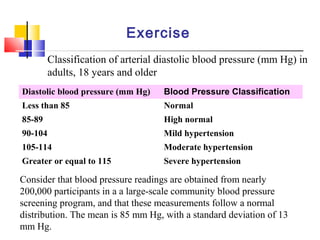
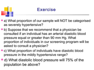
Here are the steps to solve this problem: a) Find the z-score corresponding to 115 mm Hg: (115 - 85)/13 = 2.31 The proportion that is NOT severely hypertensive is 1 - P(Z >= 2.31) = 1 - 0.0103 = 0.9897 b) Find the z-score corresponding to 90 mm Hg: (90 - 85)/13 = 0.3846 The proportion that will be asked to consult a physician is P(Z >= 0.3846) = 0.6507 c) Find the z-scores corresponding to the mildly hypertensive range: (90 - 85)/13 = 0.3846 (

1. Continuous probability
distribution

2. Recall
Continuous probability distribution
 A continuous probability distribution can assume an
infinite number of values within a given range – for
variables that take continuous values.
 The distance students travel to class.
 The time it takes an executive to drive to work.
 The length of an afternoon nap.
 The length of time of a particular phone call.
 The amount of money spent on your last haircut.

3. Normal Probability Distribution

4. Normal Probability Distribution
 The normal probability distribution is the most
important distribution for describing a continuous
random variable.
 It has been used in a wide variety of
applications:
 Heights and weights of people
 Test scores
 Scientific measurements
 Amounts of rainfall
 It is widely used in statistical inference

5. Normal Probability Distribution
 Normal Probability Density Function
where:
µ = mean
σ = standard deviation
π = 3.14159
e = 2.71828
22
2/)(
2
1
)( σµ
σπ
−−
= x
exf
This formula generates the density curve which gives
the shape of the normal distribution.

6. According to the Germans:
“That’s right on the money”
2
2
1
2
1 




 −
−
σ
µ
πσ
X
e
Herr
Gauss
The Normal distribution is also known as
the Gaussian distribution

7.  “Bell shaped” and Symmetrical
about the mean µ.
 Unimodal and its mode
occurs at x = µ.
 Mean, median and
mode are equal
 Interquartile range
equals 1.33 σ
 Random variable has infinite
range from –∞ to ∞.
 The total area under the
curve and above the horizontal axis is equal to 1.
Properties of the Normal
Distribution
µ
x
f(x)
Mean
Median
Mode

8. Most
observations in
the distribution
are close to the
mean, with
gradually fewer
observations
further away
Properties of the Normal
Distribution
µ
x
f(x)
Mean
Median
Mode

9. Properties of the Normal
Distribution
Empirical Rule
 68.3 % of all observations
lie within 1 standard
deviation of the mean
 95.4 % of all observations
lie within 2 standard
deviations of the mean
 99.7 % of all observations
lie within 3 standard
deviations of the mean
µ-3σ µ-2σ µ-1σ µ µ+1σ µ+2σ µ+3σ
68.26%
95.45%
99.74%
55 70 14585 100 115 130
µ-3σ µ-2σ µ-1σ µ µ+1σ µ+2σ µ+3σ
55 70 14585 100 115 130
For a normal distribution, the following rules hold true;
These rules are commonly
known as the Empirical Rule

10. Women participating in a three-day experimental
diet regime have been demonstrated to have
normally distributed weight loss with mean 600 g
and a standard deviation 200 g.
a) What percentage of these women will have a
weight loss between 400 and 800 g?
b) What percentage of women will lose weight too
quickly on the diet (where too much weight is
defined as >1000g)?
Application of the Empirical Rule

11. X : (600,200)
600 800 1000 12004002000
~ 68%
a)

12. X : (600,200)
600 800 1000 12004002000
b)
2.3%

13. σ2
2
2
µ x
σ1
2
1
µ µ1 < µ2
 a. The normal distribution depends on the values of the
parameters µ, the population mean and σ2, the
population variance.
 a. Two normal curves, which have the same standard
deviation but different means.
Properties of the Normal Distribution

14. σ2
2
xµ1 = µ2
σ1
2
σ2
2
σ1
2
<
b. Two normal curves with the same mean but
different standard deviations
Properties of the Normal Distribution

15. σ2
2
xµ1 < µ2
σ1
2
σ2
2
σ1
2
<
µ1
µ2
 c. Two normal curves that have different means and
different standard deviations.
Properties of the Normal Distribution

16. Areas under the Normal Curve
 The area under the curve bounded by the two ordinates x = x1
and x = x2 equals the probability that the random variable x
assumes a value between x = x1 and x = x2. Thus, for the normal
curve in the Figure below, the P(x1 < x < x2) is represented by the
area of the shaded region.
µx1 x2

17.  The area under the curve between any two ordinates
depend upon the values of µ and σ and consequently, the
probability associated with distributions differ in mean and
standard deviation will be different for the two given values
of x.
Areas under the Normal Curve
I
II
x1 x2
P(x1 < x < x2) for different Normal curves

18. Many Normal Distributions
By varying the parameters σ and µ, we
obtain different normal distributions
There are an infinite number of normal distributions

19.  It would be hopeless task to set up separate
tables of normal curve areas for every
conceivable value of µ and σ
Areas under the Normal Curve

20. Which Table to Use?
An infinite number of normal distributions means an
infinite number of tables to look up!
Yet we must use tables if we hope to avoid the
use of integral calculus

21. P(x1 < x < x2)
= ?
Finding Probabilities
Probability is the
area under the
curve!
x1 x2
X

22. Fortunately, all the observations of any normal
random variable x could be transformed to a new
set of observations of a normal random variable z
with mean zero and variance 1, by using the
transformation namely,
σ
µ−
=
X
Z
The Standard Normal Distribution

23. σ
µ z1
σ =1
0x1
z2x2
Any Normal Distribution Standard Normal Distribution
Areas will be equal.
zx
The Standard Normal Distribution
 The new distribution is called Standard Normal
Distribution, with mean equal to 0 and it’s standard
deviation equal to 1.

24.  By standardising any normally distributed random
variable, we can use just the table namely,
Areas Under the Normal Curve
Or
Areas of a Standard Normal Distribution
Such tables are usually found in the Appendix of any
statistics book.
Standard Normal Distribution
Tables

25. Learn how to use the different table

27. Entries give the probability that a standard
normally distributed random variable will assume
a value to the left of a given z value.
This means we have to sometimes perform minor
calculations to determine probabilities.
Use of the Normal Probability Table

28. Example
z .00 .01 .02 .03 .04 .05 .06 .07 .08 .09
1.5 .9332 .9345 .9357 .9370 .9382 .9394 .9406 .9418 .9429 .9441
1.6 .9452 .9463 .9474 .9484 .9495 .9505 .9515 .9525 .9535 .9545
1.7 .9554 .9564 .9573 .9582 .9591 .9599 .9608 .9616 .9625 .9633
Find the probability that z is less than 1.74.
1. Locate a value of z equal to 1.7 in the left column.
2. Move across the row to the column under 0.04, where we
read 0.9591.
Therefore,
P(z < 1.74) = 0.9591.
z

29. 1. State the problem.
2. What is the appropriate probability
statement?
3. Draw a picture and shade required area
4. Convert to a standard normal distribution
5. Find the probability in the standard normal
table
Computing Normal Probabilities

30. Example: Suppose the number of a
particular type of bacteria in samples of
1-ml of drinking water tend to be
approximately normally distributed with µ
=85 and σ2
= 81.
What is the probability that a given 1-ml
sample will contain more than 100
bacteria?

31. σ
85 100
Find this area
σ = 9
We are to find the P(x> 100)
Sketch a curve
To find the P(x> 100), we need to evaluate the area
under the normal curve to the right of x = 100.
x

32.  transform x = 100 to the corresponding z value
σ
µ−
= 1
1
x
z
Since µ = 85 and σ = 981 =
9
85100 −
=z = 1.67

33. 0 1.67
σ = 1
Find this area
z
Hence
P(x> 100) = P(z > 1.67)
Since the area to the right and the table only
gives the probability to the left of the
distribution we use
P(z > 1.67) = 1 − P(z < 1.67)

34. Z 0 0.01 0.02 0.03 0.04 0.05 0.06 0.07 0.08 0.09
1.5 0.9332 0.9345 0.9357 0.937 0.9382 0.9394 0.9406 0.9418 0.9429 0.9441
1.6 0.9452 0.9463 0.9474 0.9484 0.9495 0.9505 0.9515 0.9525 0.9535 0.9545
1.7 0.9554 0.9564 0.9573 0.9582 0.9591 0.9599 0.9608 0.9616 0.9625 0.9633
1.8 0.9641 0.9649 0.9656 0.9664 0.9671 0.9678 0.9686 0.9693 0.9699 0.9706
1.9 0.9713 0.9719 0.9726 0.9732 0.9738 0.9744 0.975 0.9756 0.9761 0.9767

35. 0 1.67
σ = 1
Find this area
z
Hence
P(x> 100) = P(z > 1.67)
Since the area to the right and the table only gives the
probability to the left of the distribution we use
P(z > 1.67) = 1 − P(z < 1.67)
= 1 − 0.9525 = 0.0475.
So 1-ml sample will has 0.0475 probability to contain more
than 100 bacteria

36. Exercise
If the total cholesterol values for a certain target population
are approximately normally distributed with a mean of 200
(mg/100 mL) and a standard deviation of 20 (mg/100 mL),
What is the probability that a person picked at random from
this population will have a cholesterol value greater than 240
(mg/100 mL)?
Answer = 0.0228

37. Example 2
IQ scores (IQ is Intelligence Quotient) on the
Wechsler Adult Intelligence Scale are
approximately normally distributed with mean µ =
100 and σ = 15.
a. What is the proportion of persons having IQs
between 80 and 120?

38. Solution
Let x1 = 80 and x2 = 120
This question means that we are to find the probability
P(x1<IQ<x2) = P(80< IQ <120)
Sketch a normal curve like the one in the figure below.
Shade in the area desired.
σ =15
10080 120 x
Example 2 cont.

39. Find the z values corresponding to x1 = 80 and x2 = 120
Example 2 cont.
Since, P(x1<x<x2) =P (z1<z<z2)
Therefore, P(80<IQ<120) = P(−1.33<z<1.33)

40. The P(−1.33<z<1.33) is given by the area of the shaded region
in the figure. This area may be found by subtracting the area
to the left of the ordinate z = −1.33 from the entire area to the
left of z = 1.33.
Example 2 cont.
σ = 1
0-1.33 1.33 z

41. P(80<IQ<120) = P(−1.33<z<1.33)
= P(z<1.33) − P(z<−1.33)
= 0.9082 – 0.0918
= 0.8164.
Therefore the proportion of persons
having IQs between 80 and 120
is 0.8164, about 82%.
σ =1
0-1.33 1.33 z

42. Example 3
Suppose that the hemoglobin levels for healthy adult males
are approximately normally distributed with a mean of 16
and variance of 0.81. Find the probability that a randomly
chosen healthy adult male has a hemoglobin level less than
14.
Solution
We are to find P(x < 14)
Since µ = 16 and σ = = 0.9
We find Z = − 2.22
P(x < 14) = P(Z < − 2.22)
= 0.0132
Therefore, only about 1.3% of healthy adult males have
σ=0.81
σ= 1
16
0
14
-2.22
x
z

44. .
Inverse Normal Distribution
Finding x value when probabilities
(areas) are given

45. 1. State the problem
2. Draw a picture
3. Use table to find the probability closest to the one you
need
4. Read off the z-value
5. Unstandardise i.e. x = µ + zσ
Finding a Value (X) given a Probability

46. Example
Given a normal distribution with µ = 40 and σ = 6,
find the value of x that has
a. 45% of the area below it
b. 14% of the area above it.
Solution
In this problem we reverse the process and begin
with a known area or probability, find the z value,
and then determine x by rearranging the formula
to give
σ
µ−
=
x
z µσ += zx

48. a. We require a z value that leaves an area of 0.45 to the left.
From the table we find P(z < -0.13) = 0.45 so that the desired
z value is -0.13.
σ=6
40 x
0.45
µσ += zx
= (-0.13 X 6 )+ 40 = 39.22
x =?
Example cont.

49. b. 14% of the area above it.
This time we require a z value that leaves 0.14 of the area to
the right and hence an area of 0.86 to the left.
From the table we find P(z < 1.08) = 0.86
so that the desired z value is 1.08 and
x = (6)(1.08) + 40
= 46.48
σ =6
x =?
0.86
40
µσ += zx
Example cont.
0.14

51. Classification of arterial diastolic blood pressure (mm Hg) in
adults, 18 years and older
Consider that blood pressure readings are obtained from nearly
200,000 participants in a a large-scale community blood pressure
screening program, and that these measurements follow a normal
distribution. The mean is 85 mm Hg, with a standard deviation of 13
mm Hg.
Diastolic blood pressure (mm Hg) Blood Pressure Classification
Less than 85 Normal
85-89 High normal
90-104 Mild hypertension
105-114 Moderate hypertension
Greater or equal to 115 Severe hypertension
Exercise

52. a) What proportion of our sample will NOT be categorised
as severely hypertensive?
b) Suppose that we recommend that a physician be
consulted if an individual has an arterial diastolic blood
pressure equal or greater than 90 mm Hg. What
proportion of individuals in our screening program will be
asked to consult a physician?
c) What proportion of individuals have diastolic blood
pressure in the mildly hypertensive range?
d) What diastolic blood pressure will 75% of the
population be above?
Exercise

53. EXERCISE
(a) The distribution of serum levels of alpha tocopherol
(serum vitamin E) is approximately normal with mean
860 mg/dL and standard deviation 340mg/dL.
What serum level will 85% of the population be
below?
(b) Suppose a person is identified as having toxic
levels of alpha tocopherol if his or her serum level is
greater than 2000mg/dL. What percentage of people
will be so identified?

54. Under certain conditions, a binomial random
variable has a distribution that is approximately
normal.
Normal approximation of the
Binomial Distribution

55. If n, p, and q are such
that:
np and nq
are both greater than
5.
We use a normal distribution with
qpnandpn =σ=µ
Normal approximation of the
Binomial Distribution

56. Application of Normal Distribution
If 22% of all patients with high blood pressure
have side effects from a certain medication, and
100 patients are treated, find the probability that
at least 30 of them will have side effects.
Using the Binomial Probability Formula we would need
to compute:
P(30) + P(31) + ... + P(100) or 1 − P( x < 29)

57. Using the Normal Approximation to
the Binomial Distribution
Check if Is it appropriate to use the normal
distribution?
n p = 22
n q = 78
Both are greater than five.

58. Find the mean and standard deviation
µ = n p = 100(.22) = 22
and σ =
14.416.17
)78)(.22(.100
=
=
qpnandpn =σ=µ
Using the Normal Approximation to
the Binomial Distribution

59. σ
22 30
Find this area
To find the probability that at least 30 of
them will have side effects, find P( x ≥ 30)
σ = 4.14
Using the Normal Approximation to the
Binomial Distribution

60. Applying the Normal Distribution
z = 30 – 22 = 1.81
4.14
Find P( z ≥ 1.81) = 1 – P (z < 1.81) = 0.0351
0 1.81
The probability that at least 30 of the patients will have side
effects is 0.0351.
σσ = 1