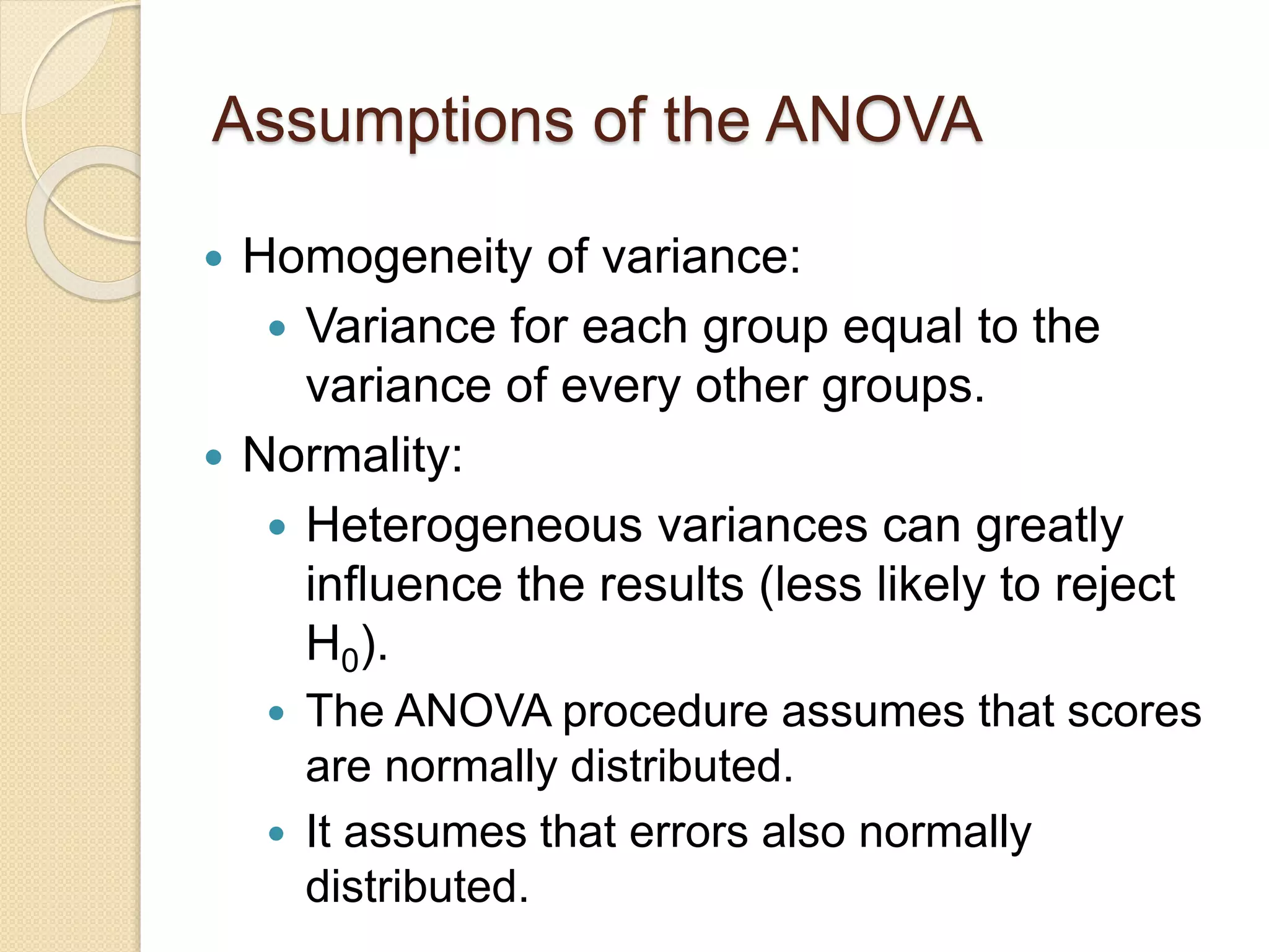
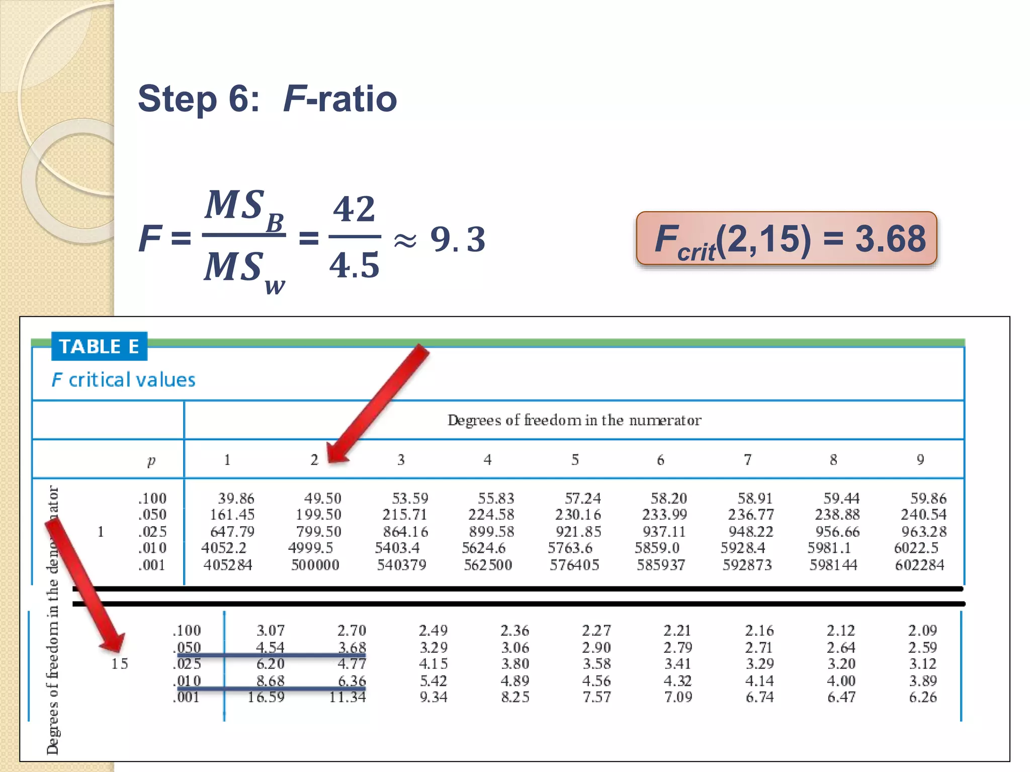
ANOVA (F test)
and
Mean Differentiation Tests
Dr. S. Parasuraman, Faculty of Pharmacy, AIMST University.
Father of
modern statistics
Sir Ronald
Aylmer Fisher
Compare means (or medians)
Number of group(S) Test recommended
One Group One sample t test
Wilcoxon rank sum test
Two groups Unpaired t test
Paired t test
Mann-Whitney test
Welch’s corrected t test
Wilcoxon matched pair test
3-26 groups One-way ANOVA
Repeated measures ANOVA
Kruskal-Wallis test
Friedman test
Difference between t test and
ANOVA
T-test ANOVA
Dependent Interval or ratio
variable
Interval or ratio variable
Independent Binary variable with
only two groups
Categorical variable
Null hypothesis H0 : µ1 = µ2
HA : µ1 ≠ µ2
H0 : µ1 =µ2= µ3 or
H0 : µ1 =µ2=µ3=µ4… = HJ
HA : The mean are not
equal
Probable
distribution
T distribution F distribution
Analysis of variance (ANOVAs)
 ANOVAs are useful for comparing three or
more means (groups or variables) for
statistical significance.
 ANOVAs is similar to multiple two-sample t-
tests with less type I error.
 Continuous response variable and at least one
categorical factor must be there to perform
ANOVA.
 ANOVAs require data from normally distributed
populations with equal variances between
factor levels.
Types of errors
Judgment of null
hypothesis (H0)
Valid/ True Invalid/ False
Reject Type I error
(false positive)
Correct
inference
(True positive)
Fail to reject Correct
inference
(True negative)
Type II error
(false negative)
100 Kg10
Kg 100 Kg
100 KgType I error
Type II error
Types of ANOVA
ANOVA type Design properties
One-way One fixed which can have either an unequal or
equal number of observations per treatment.
Balanced Model may contain any number of fixed and
random factors.
General linear model Expands on Balanced ANOVAs by allowing
unbalanced designs and covariates (continuous
variables).
 One-way ANOVA
 Factorial ANOVA
 Repeated measures
 Multivariate analysis of
variance
One-way ANOVA
 It is used to test for differences among two or more
independent (unrelated) means (groups). When
there are only two means to compare, the t-test and
the ANOVA F-test are equivalent; the relation
between ANOVA and t is given by F = t2.
Assumptions
 The populations from which the samples were obtained
must be normally or approximately normally distributed.
 The samples must be independent.
 The variances of the populations must be equal.
E.g.: Different levels of blood glucose in 3 groups of
population.
Factorial ANOVA
 Factorial ANOVA is analysis of variance
involving two or more independent
variables or predictors.
 Two-way ANOVA is an example of factorial ANOVA
in which the effect of two independent variables on
the dependent variable.
Independent variables
I 2+
Dependent
variables
1 One-way
ANOVA
Factorial ANOVA
2+ Multiple ANOVA MANOVA
MANOVA: Multivariate Analysis of Variance
Procedure for Two-way
Analysis
Repeated measures
 Repeated measures ANOVA is the equivalent
of the one-way ANOVA, but for related, not
independent groups, and is the extension of
the dependent t-test. A repeated measures
ANOVA is also referred to as a within-subjects
ANOVA or ANOVA for correlated samples.
Levels of Blood glucose at different time point form same animals
Level
1
Level
2
Level
3
Level
4
Levels (related groups) of the
independent variable ‘Time’
Group I
Control
Group III
Treatment
Group II
Treatment
Compare the effect the
treatment(s) on blood
glucose level at various time
intervals.
Multivariate analysis of variance
 Multivariate analysis of variance (MANOVA) is
a generalized form of univariate ANOVA with
several dependent variables.
Assumptions of the ANOVA
 Homogeneity of variance:
 Variance for each group equal to the
variance of every other groups.
 Normality:
 Heterogeneous variances can greatly
influence the results (less likely to reject
H0).
 The ANOVA procedure assumes that scores
are normally distributed.
 It assumes that errors also normally
distributed.
Assumptions of the ANOVA
 Independence of Observations:
 The scores for one group are not
dependent on the scores from another
group.
 The Null Hypothesis
Assumptions of the ANOVA
Heterogeneous variances can greatly
influence the results
F-distribution/ Snedecor's F distribution/
Fisher–Snedecor distribution
Characteristics of the F-Distribution
 F-distributions are generally not symmetric and skewed to
the right.
 The values of F can be 0 or positive, but they cannot be
negative.
 There is a different F distribution for each pair of degrees of
freedom for the numerator and denominator.
 The shape of the F-distribution depends upon the degrees of
freedom in the numerator and denominator.
Relationship Between the F Test
Statistic and P-ValueCompare the same
means
F here
Large F test
statistic, small P-
value
F here
Small F test statistic,
large P-value
Fail to reject equality
of population means.
Reject equality of
population means
At least one sample
mean is very
different.
Sample
means are
all close
Example
Objective: To study the effect three different
fertilizer on plant growth (n= 6/ group).
The null hypothesis (H0) says three different
fertilizer produce same response, on average
a1 a2 a3
6 8 13
8 12 9
4 9 11
5 11 8
3 6 7
4 8 12
Step I: Calculate the mean within group
𝑌1 =
1
6
𝑌1𝑖 =
6+8+4+5+3+4
6
= 5
𝑌2 =
1
6
𝑌2𝑖 =
8+12+9+11+6+8
6
= 9
𝑌3 =
1
6
𝑌3𝑖 =
13+9+11+8+7+12
6
= 10
Step 2: Calculate the over all mean
𝑌 =
𝑖 𝑌
𝑎
=
𝑌1 +𝑌2+𝑌3
𝑎
=
5+9+10
3
= 8
Step 3: Calculate the ‘between-group’ sum of
squared differences:
𝑆 𝐵 = n(𝑌1 − 𝑌)2
+ n(𝑌2 − 𝑌)2
+ n(𝑌3 − 𝑌)2
= 6(5 - 8)2 + 6(9 - 8)2 + 6(10 - 8)2 = 84
*n= number of variables in the group
Step 4: Calculate “degree of freedom” and mean
“square value”
 Degree of freedom (DF) = number of group-1
 Mean square value (MSB) = sum of squared
differences/ DF
DF= 3-1 = 2
MSB = 84/2 = 42
Step 5: Calculate “within-group” sum of squares
(Sw)
 Sw = (1)2+(3)+(-1)+(0)+(-2)+(-1)+(-1)+(3)+(0)+
(2)+ (-3)+ (-1)+(3)+(-1)+(1)+(-2)+(-3)+(2) = 68
 Within group DF = fw = a(n-1) = 3(6-1) = 15
 Within group mean square value is MSw=Sw/fw
= 68/15 ≈ 𝟒. 𝟓
a1 a2 a3
6-5=1 8-9=-1 13-10=3
8-5=3 12-9=3 9-10=-1
4-5=-1 9-9=0 11-10=1
5-5=0 11-9=2 8-10=-2
3-5=-2 6-9=-3 7-10=-3
4-5=-1 8-9=-1 12-10=2
Step 6: F-ratio
F =
𝑴𝑺 𝑩
𝑴𝑺 𝒘
=
𝟒𝟐
𝟒.𝟓
≈ 𝟗. 𝟑 Fcrit(2,15) = 3.68
Fcrit(2,15) = 3.68 ; Since 9.3 > 3.68 the result is
significant at 0.50 i.e., p<0.05.
Post-hoc test: (from Latin post hoc “after this)
Post hoc test are run to conform where the
differences occurred between groups. It is
usually concerned with finding patterns and
relationship between sub-groups of sampled
population.

Anova (f test) and mean differentiation

  • 1.
    ANOVA (F test) and MeanDifferentiation Tests Dr. S. Parasuraman, Faculty of Pharmacy, AIMST University. Father of modern statistics Sir Ronald Aylmer Fisher
  • 2.
    Compare means (ormedians) Number of group(S) Test recommended One Group One sample t test Wilcoxon rank sum test Two groups Unpaired t test Paired t test Mann-Whitney test Welch’s corrected t test Wilcoxon matched pair test 3-26 groups One-way ANOVA Repeated measures ANOVA Kruskal-Wallis test Friedman test
  • 3.
    Difference between ttest and ANOVA T-test ANOVA Dependent Interval or ratio variable Interval or ratio variable Independent Binary variable with only two groups Categorical variable Null hypothesis H0 : µ1 = µ2 HA : µ1 ≠ µ2 H0 : µ1 =µ2= µ3 or H0 : µ1 =µ2=µ3=µ4… = HJ HA : The mean are not equal Probable distribution T distribution F distribution
  • 4.
    Analysis of variance(ANOVAs)  ANOVAs are useful for comparing three or more means (groups or variables) for statistical significance.  ANOVAs is similar to multiple two-sample t- tests with less type I error.  Continuous response variable and at least one categorical factor must be there to perform ANOVA.  ANOVAs require data from normally distributed populations with equal variances between factor levels.
  • 5.
    Types of errors Judgmentof null hypothesis (H0) Valid/ True Invalid/ False Reject Type I error (false positive) Correct inference (True positive) Fail to reject Correct inference (True negative) Type II error (false negative) 100 Kg10 Kg 100 Kg 100 KgType I error Type II error
  • 6.
    Types of ANOVA ANOVAtype Design properties One-way One fixed which can have either an unequal or equal number of observations per treatment. Balanced Model may contain any number of fixed and random factors. General linear model Expands on Balanced ANOVAs by allowing unbalanced designs and covariates (continuous variables).  One-way ANOVA  Factorial ANOVA  Repeated measures  Multivariate analysis of variance
  • 7.
    One-way ANOVA  Itis used to test for differences among two or more independent (unrelated) means (groups). When there are only two means to compare, the t-test and the ANOVA F-test are equivalent; the relation between ANOVA and t is given by F = t2. Assumptions  The populations from which the samples were obtained must be normally or approximately normally distributed.  The samples must be independent.  The variances of the populations must be equal. E.g.: Different levels of blood glucose in 3 groups of population.
  • 8.
    Factorial ANOVA  FactorialANOVA is analysis of variance involving two or more independent variables or predictors.  Two-way ANOVA is an example of factorial ANOVA in which the effect of two independent variables on the dependent variable. Independent variables I 2+ Dependent variables 1 One-way ANOVA Factorial ANOVA 2+ Multiple ANOVA MANOVA MANOVA: Multivariate Analysis of Variance
  • 9.
  • 10.
    Repeated measures  Repeatedmeasures ANOVA is the equivalent of the one-way ANOVA, but for related, not independent groups, and is the extension of the dependent t-test. A repeated measures ANOVA is also referred to as a within-subjects ANOVA or ANOVA for correlated samples.
  • 11.
    Levels of Bloodglucose at different time point form same animals Level 1 Level 2 Level 3 Level 4 Levels (related groups) of the independent variable ‘Time’ Group I Control Group III Treatment Group II Treatment Compare the effect the treatment(s) on blood glucose level at various time intervals.
  • 12.
    Multivariate analysis ofvariance  Multivariate analysis of variance (MANOVA) is a generalized form of univariate ANOVA with several dependent variables.
  • 13.
    Assumptions of theANOVA  Homogeneity of variance:  Variance for each group equal to the variance of every other groups.  Normality:  Heterogeneous variances can greatly influence the results (less likely to reject H0).  The ANOVA procedure assumes that scores are normally distributed.  It assumes that errors also normally distributed.
  • 14.
    Assumptions of theANOVA  Independence of Observations:  The scores for one group are not dependent on the scores from another group.  The Null Hypothesis
  • 15.
    Assumptions of theANOVA Heterogeneous variances can greatly influence the results
  • 16.
    F-distribution/ Snedecor's Fdistribution/ Fisher–Snedecor distribution Characteristics of the F-Distribution  F-distributions are generally not symmetric and skewed to the right.  The values of F can be 0 or positive, but they cannot be negative.  There is a different F distribution for each pair of degrees of freedom for the numerator and denominator.  The shape of the F-distribution depends upon the degrees of freedom in the numerator and denominator.
  • 17.
    Relationship Between theF Test Statistic and P-ValueCompare the same means F here Large F test statistic, small P- value F here Small F test statistic, large P-value Fail to reject equality of population means. Reject equality of population means At least one sample mean is very different. Sample means are all close
  • 18.
  • 19.
    Objective: To studythe effect three different fertilizer on plant growth (n= 6/ group). The null hypothesis (H0) says three different fertilizer produce same response, on average a1 a2 a3 6 8 13 8 12 9 4 9 11 5 11 8 3 6 7 4 8 12
  • 20.
    Step I: Calculatethe mean within group 𝑌1 = 1 6 𝑌1𝑖 = 6+8+4+5+3+4 6 = 5 𝑌2 = 1 6 𝑌2𝑖 = 8+12+9+11+6+8 6 = 9 𝑌3 = 1 6 𝑌3𝑖 = 13+9+11+8+7+12 6 = 10
  • 21.
    Step 2: Calculatethe over all mean 𝑌 = 𝑖 𝑌 𝑎 = 𝑌1 +𝑌2+𝑌3 𝑎 = 5+9+10 3 = 8
  • 22.
    Step 3: Calculatethe ‘between-group’ sum of squared differences: 𝑆 𝐵 = n(𝑌1 − 𝑌)2 + n(𝑌2 − 𝑌)2 + n(𝑌3 − 𝑌)2 = 6(5 - 8)2 + 6(9 - 8)2 + 6(10 - 8)2 = 84 *n= number of variables in the group
  • 23.
    Step 4: Calculate“degree of freedom” and mean “square value”  Degree of freedom (DF) = number of group-1  Mean square value (MSB) = sum of squared differences/ DF DF= 3-1 = 2 MSB = 84/2 = 42
  • 24.
    Step 5: Calculate“within-group” sum of squares (Sw)  Sw = (1)2+(3)+(-1)+(0)+(-2)+(-1)+(-1)+(3)+(0)+ (2)+ (-3)+ (-1)+(3)+(-1)+(1)+(-2)+(-3)+(2) = 68  Within group DF = fw = a(n-1) = 3(6-1) = 15  Within group mean square value is MSw=Sw/fw = 68/15 ≈ 𝟒. 𝟓 a1 a2 a3 6-5=1 8-9=-1 13-10=3 8-5=3 12-9=3 9-10=-1 4-5=-1 9-9=0 11-10=1 5-5=0 11-9=2 8-10=-2 3-5=-2 6-9=-3 7-10=-3 4-5=-1 8-9=-1 12-10=2
  • 25.
    Step 6: F-ratio F= 𝑴𝑺 𝑩 𝑴𝑺 𝒘 = 𝟒𝟐 𝟒.𝟓 ≈ 𝟗. 𝟑 Fcrit(2,15) = 3.68
  • 27.
    Fcrit(2,15) = 3.68; Since 9.3 > 3.68 the result is significant at 0.50 i.e., p<0.05. Post-hoc test: (from Latin post hoc “after this) Post hoc test are run to conform where the differences occurred between groups. It is usually concerned with finding patterns and relationship between sub-groups of sampled population.

Editor's Notes

  • #26 DF= 3-1 = 2 Within group DF = fw = a(n-1) = 3(6-1) = 15
  • #28 DF= 3-1 = 2 Within group DF = fw = a(n-1) = 3(6-1) = 15 https://en.wikipedia.org/wiki/F-test