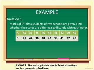
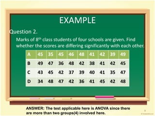
Downloaded 179 times


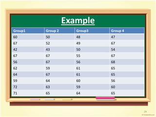
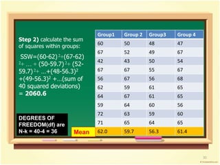
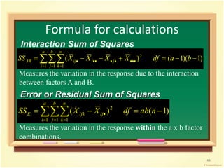
![Group1 Group 2 Group3 Group 4
60 50 48 47
67 52 49 67
42 43 50 54
67 67 55 67
56 67 56 68
62 59 61 65
64 67 61 65
59 64 60 56
72 63 59 60
71 65 64 65
62.0 59.7 56.3 61.4
Step 1) calculate the sum
of squares between
groups:
Grand mean= 59.85
SSB = [(62-59.85)2 +
(59.7-59.85)2 + (56.3-
59.85)2 + (61.4-59.85)2]
x n per group =
19.65x10 = 196.5
Mean
DEGREES OF
FREEDOM(df) are
k-1 = 4-1 = 3
30](https://image.slidesharecdn.com/analysisofvariance-140902092554-phpapp01/85/Analysis-of-variance-29-320.jpg)

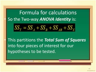
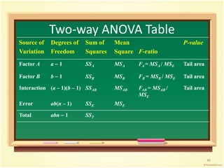
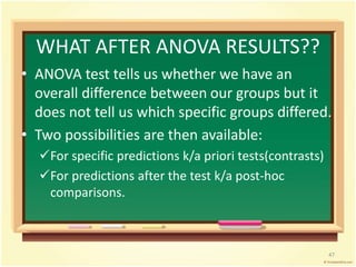


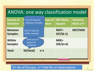
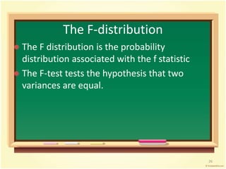
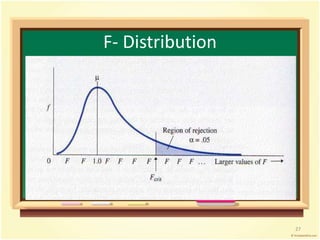
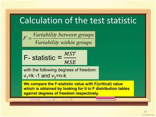
This document provides an overview of analysis of variance (ANOVA). It begins by defining parametric tests and discussing the assumptions of ANOVA. The key ideas of ANOVA are introduced, including comparing the variance between groups to the variance within groups. Calculations for one-way ANOVA are demonstrated, including sums of squares, mean squares, and the F-statistic. Examples are provided to illustrate one-way ANOVA calculations and interpretations. Violations of assumptions and extensions to two-way ANOVA are also discussed.