Download as PDF, PPTX
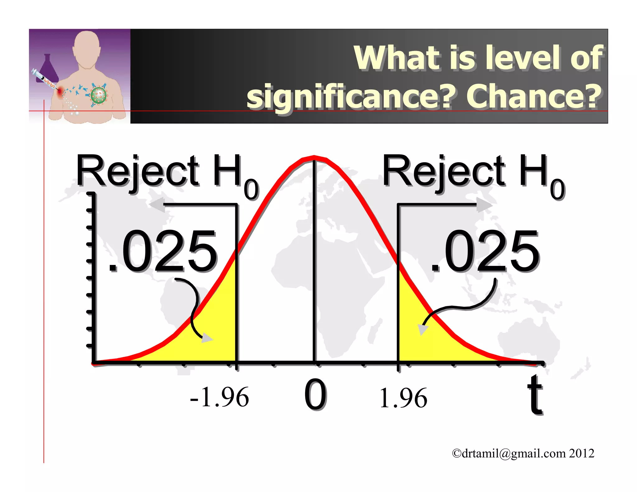
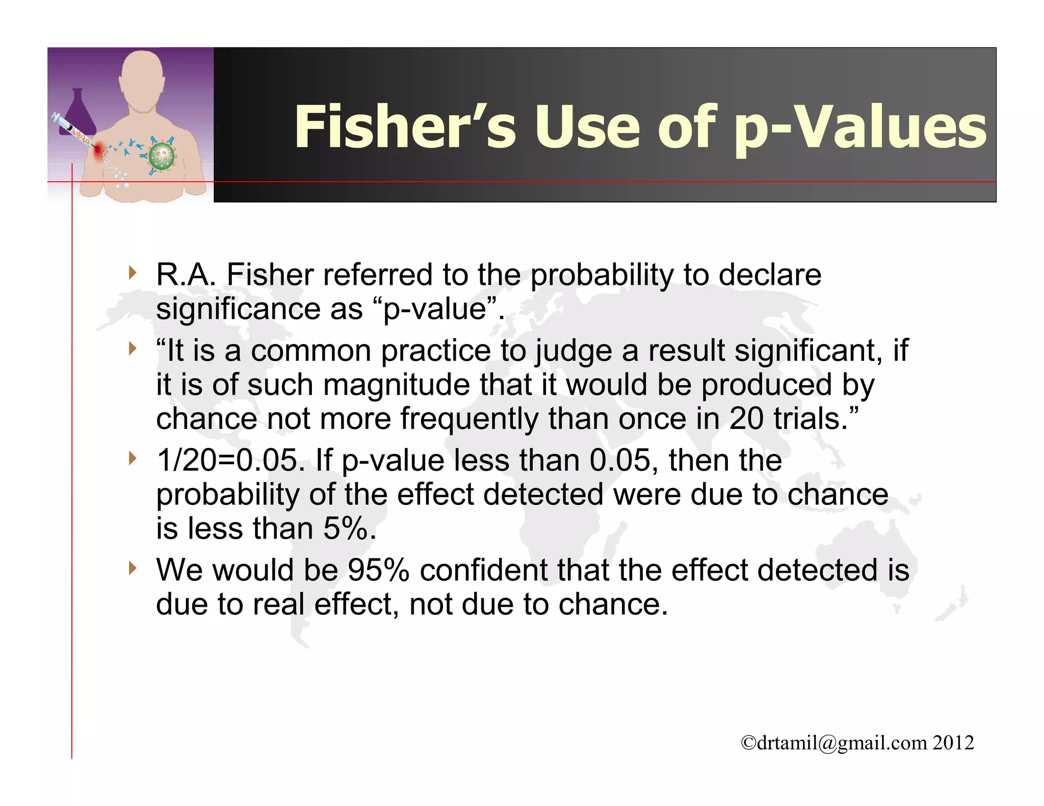
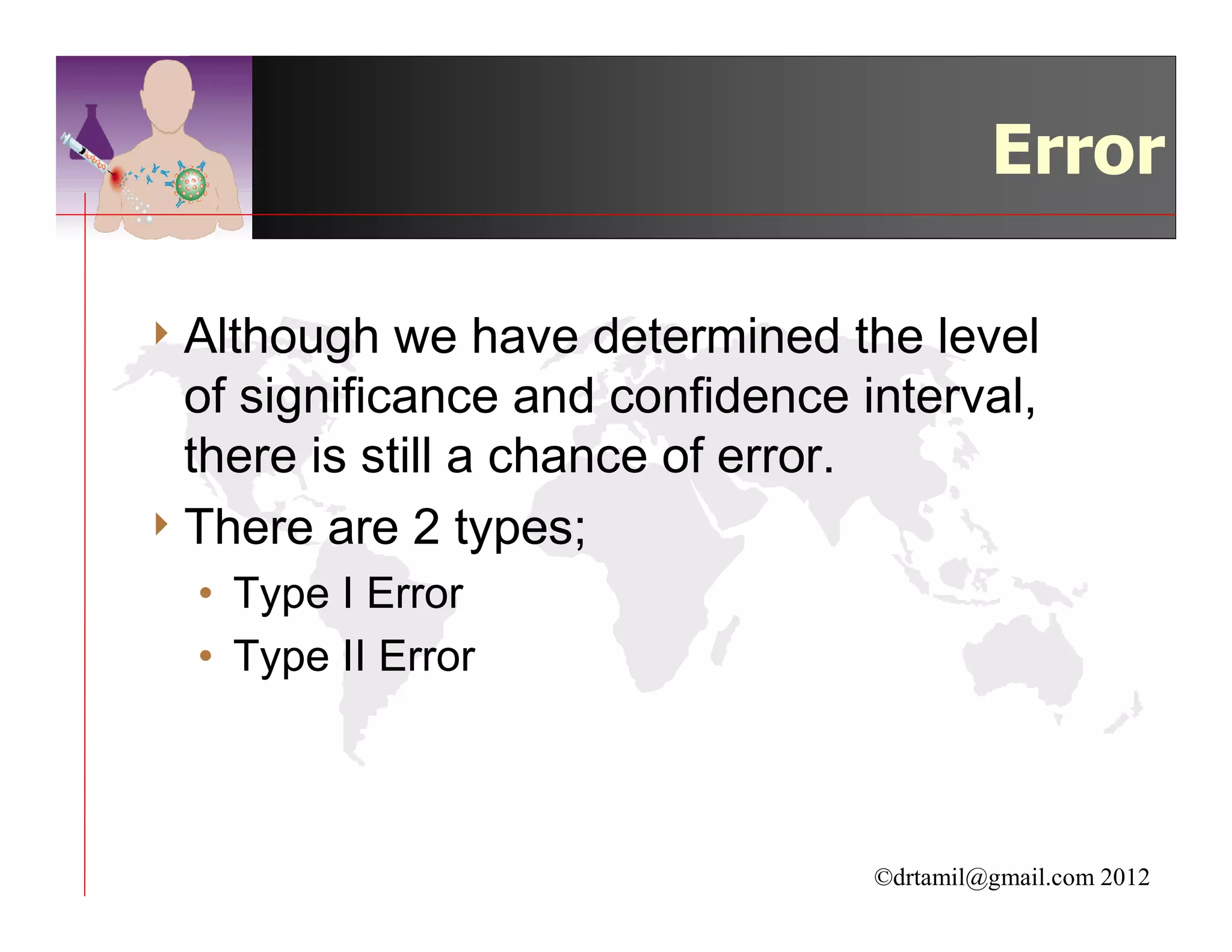
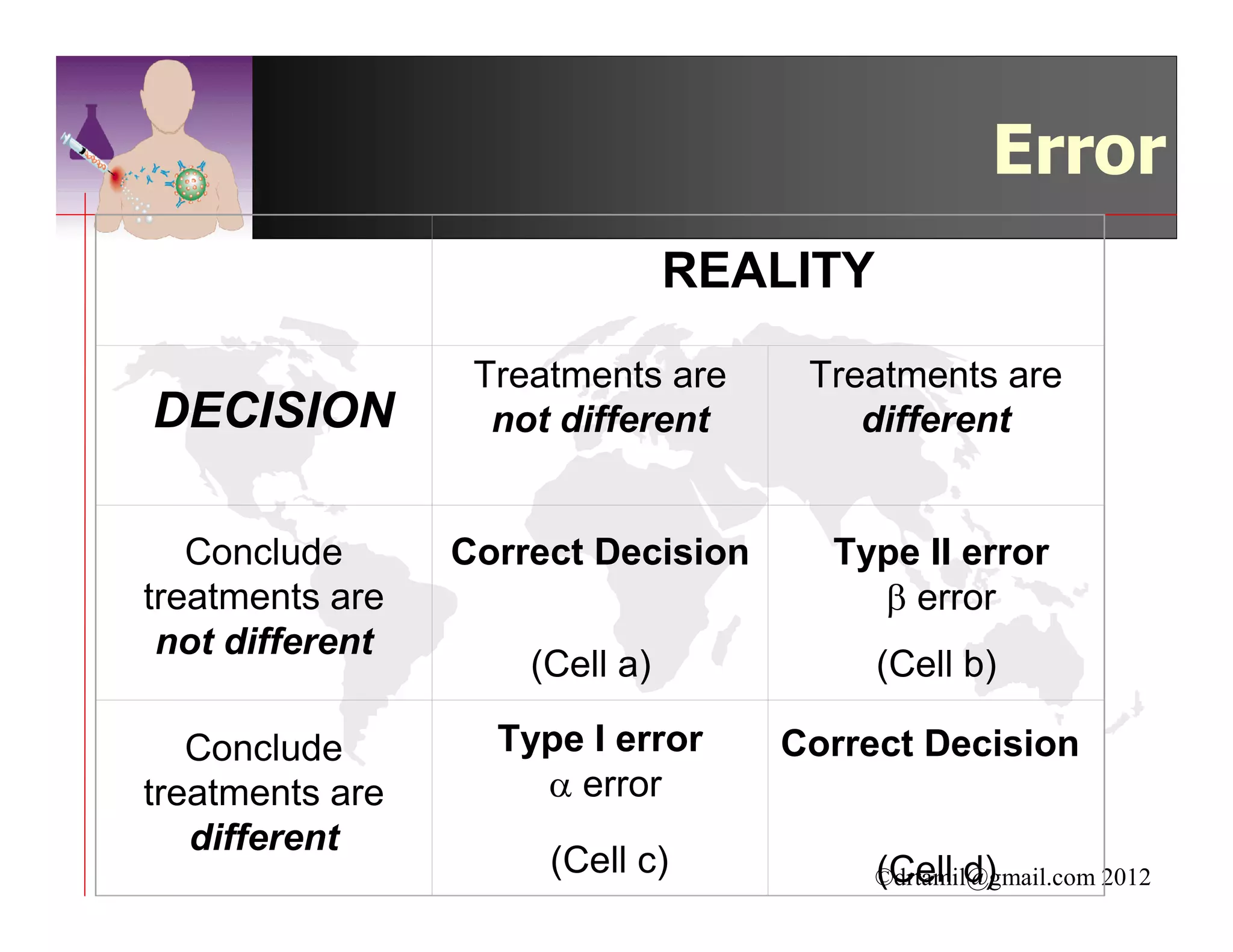
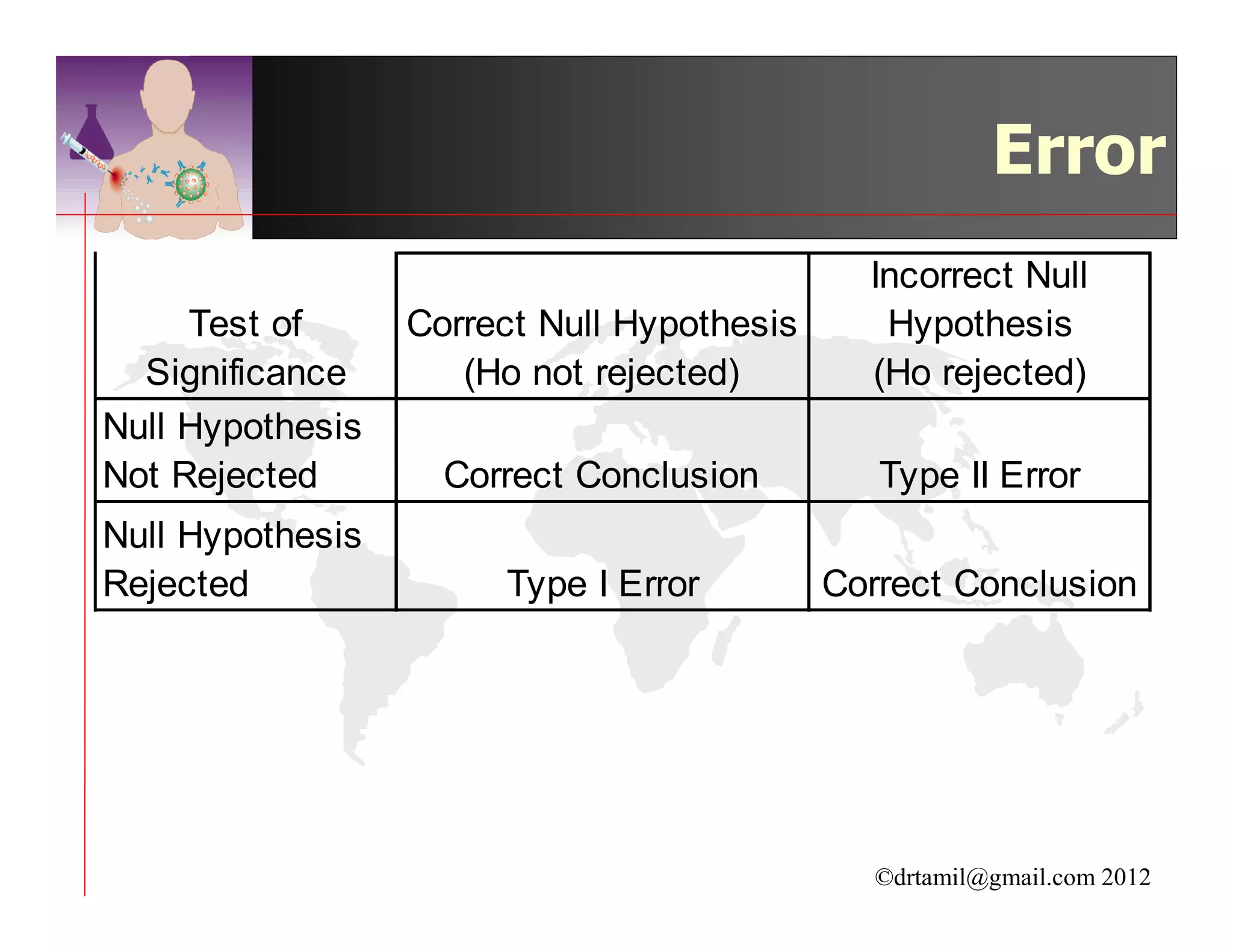
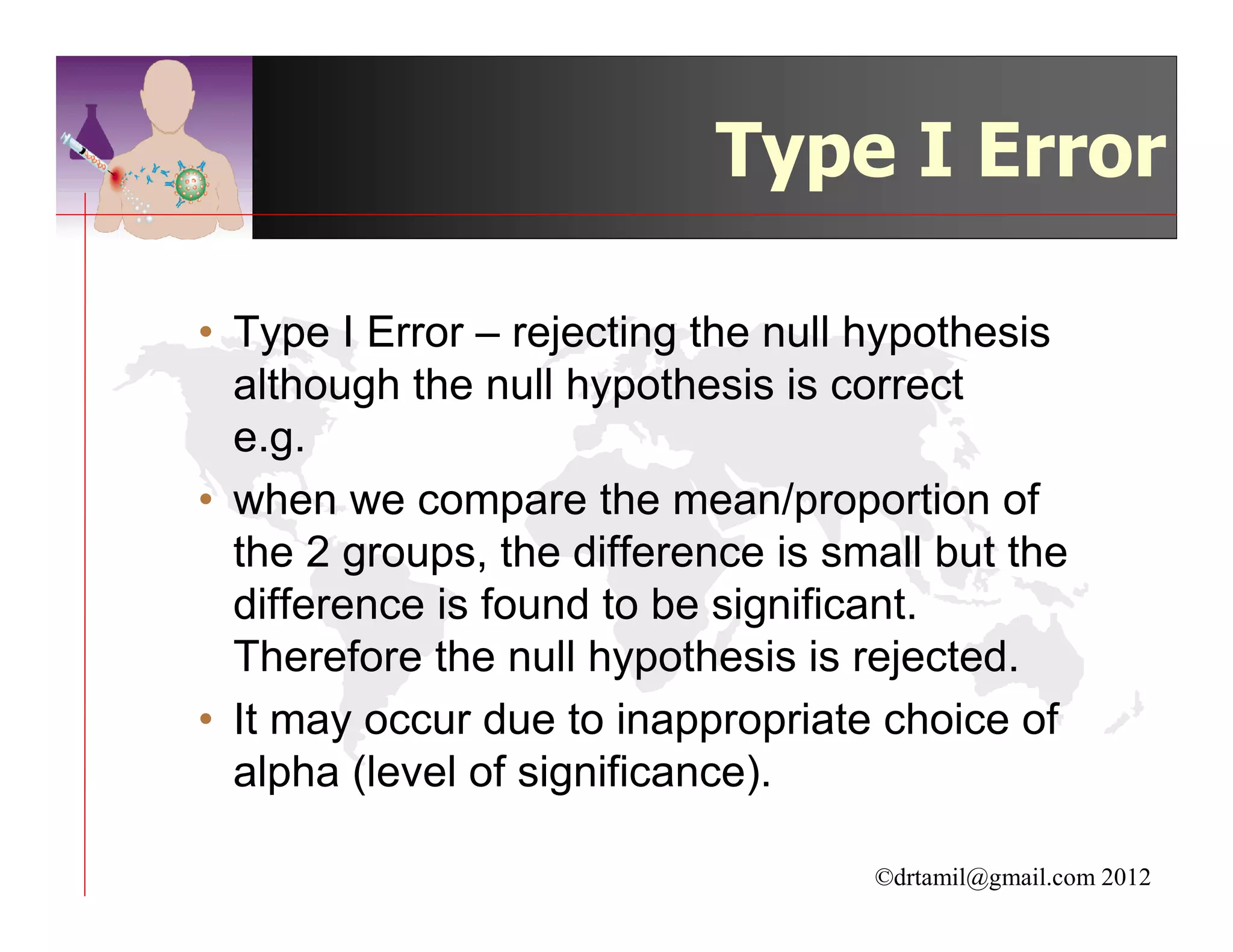
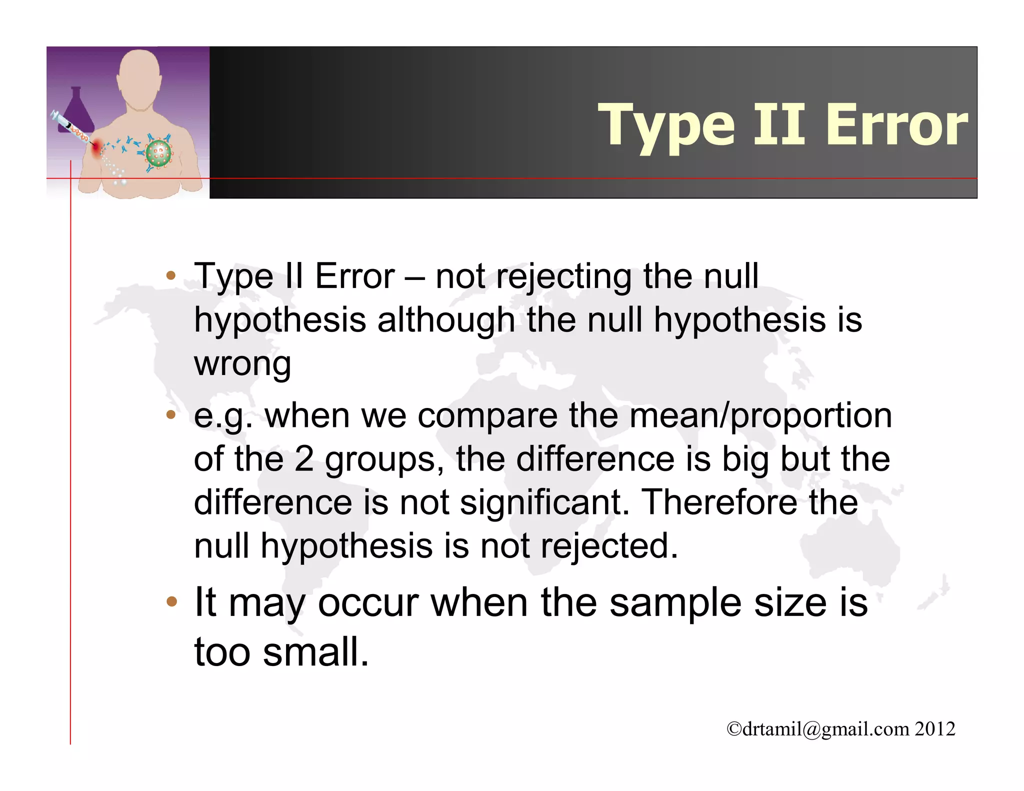
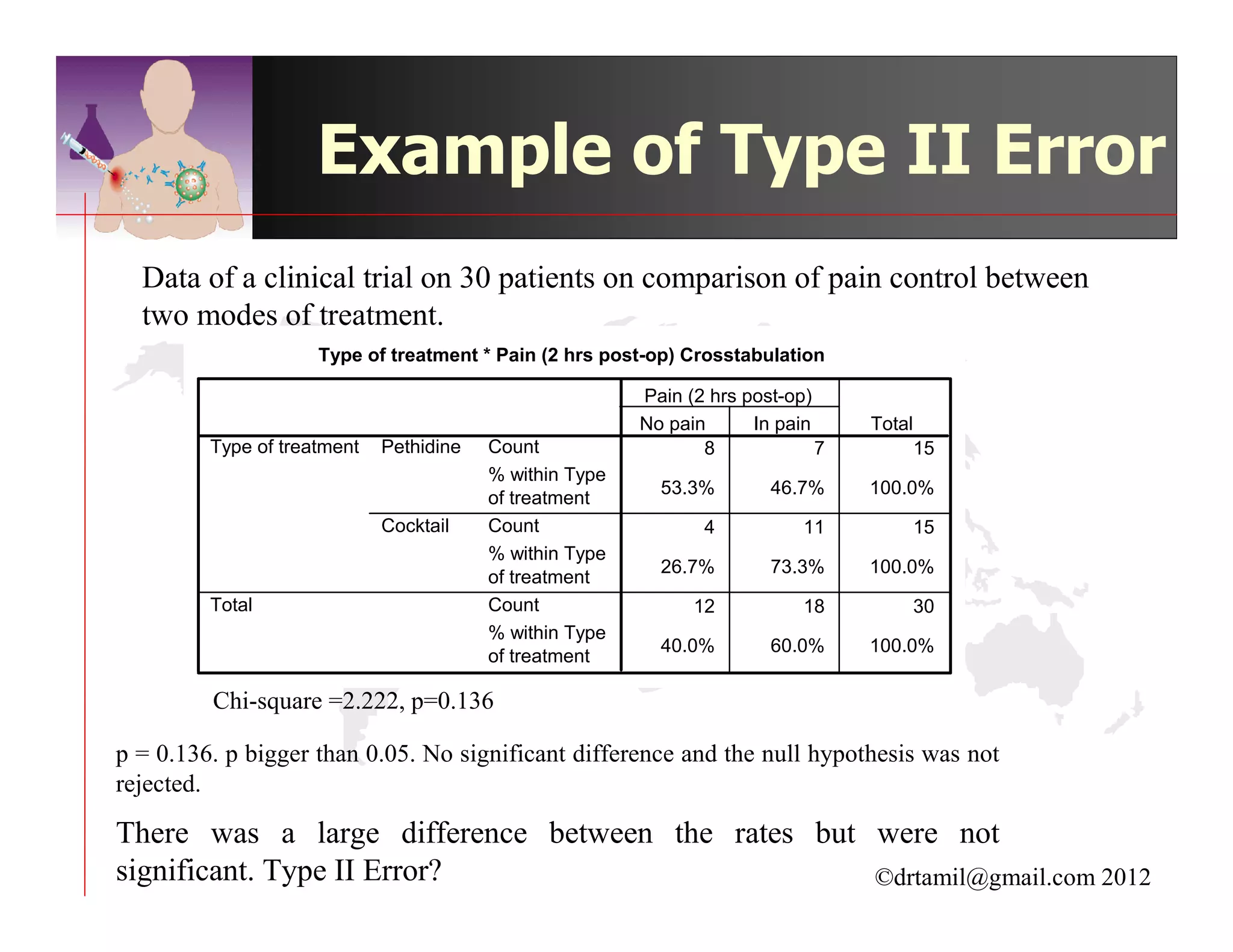

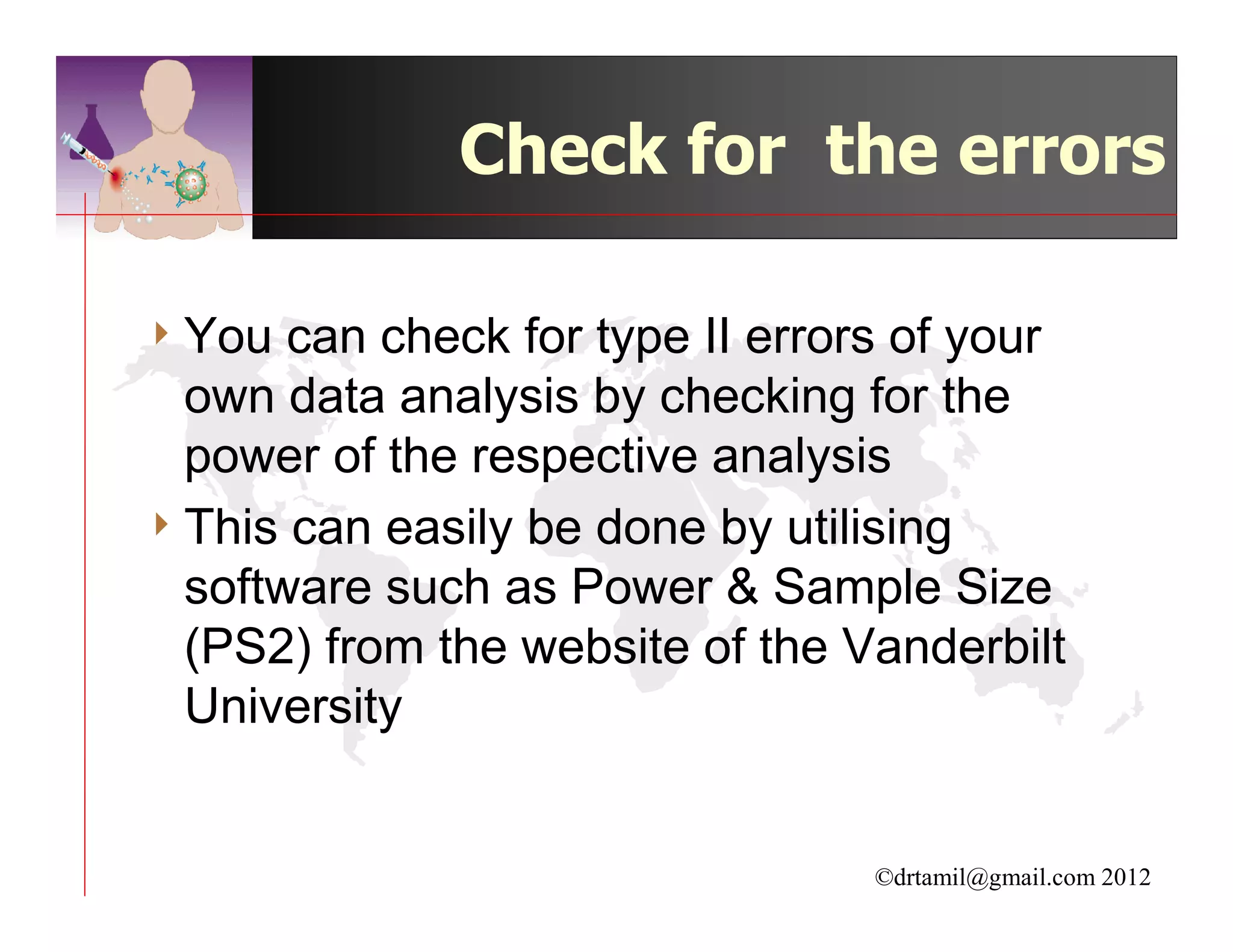
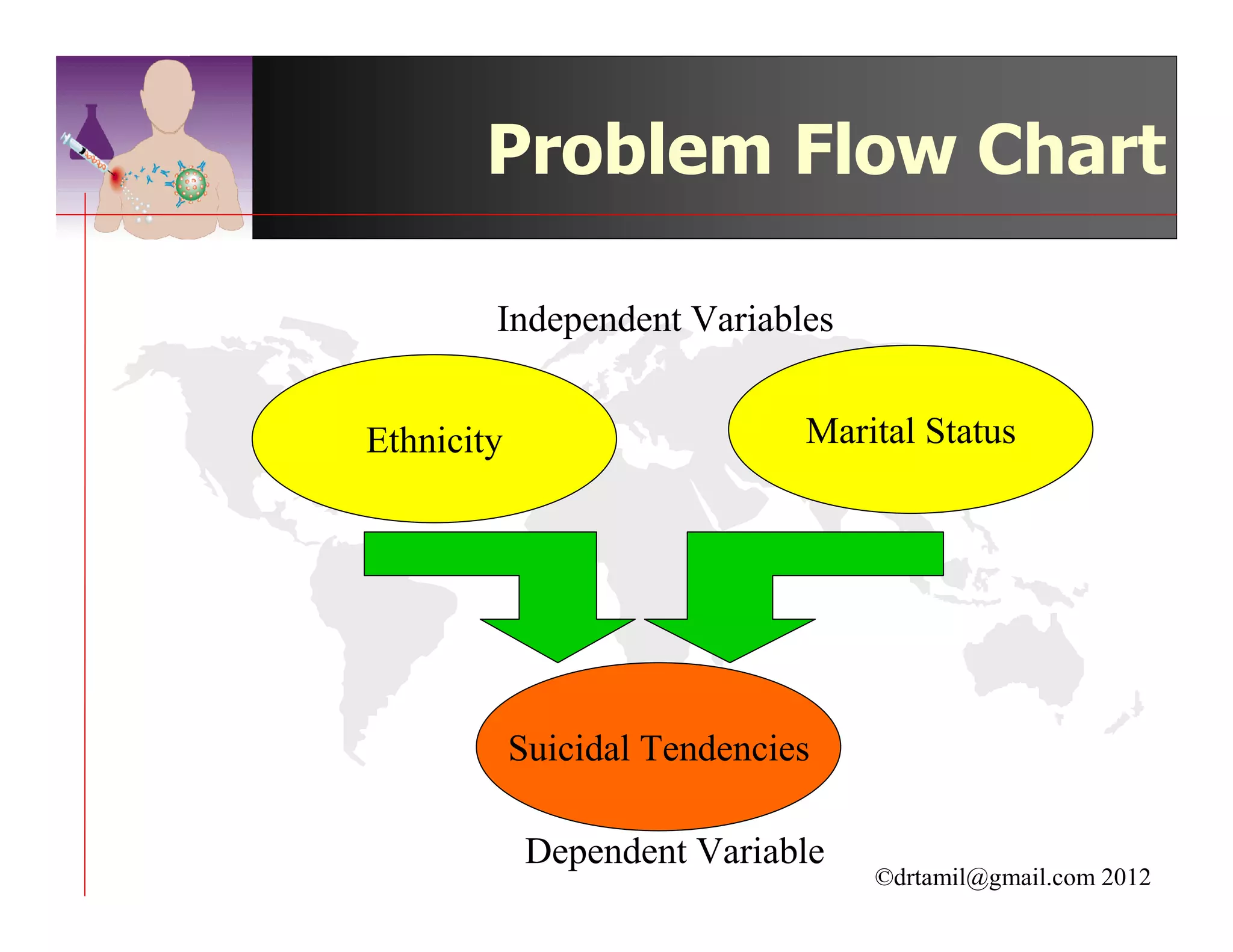
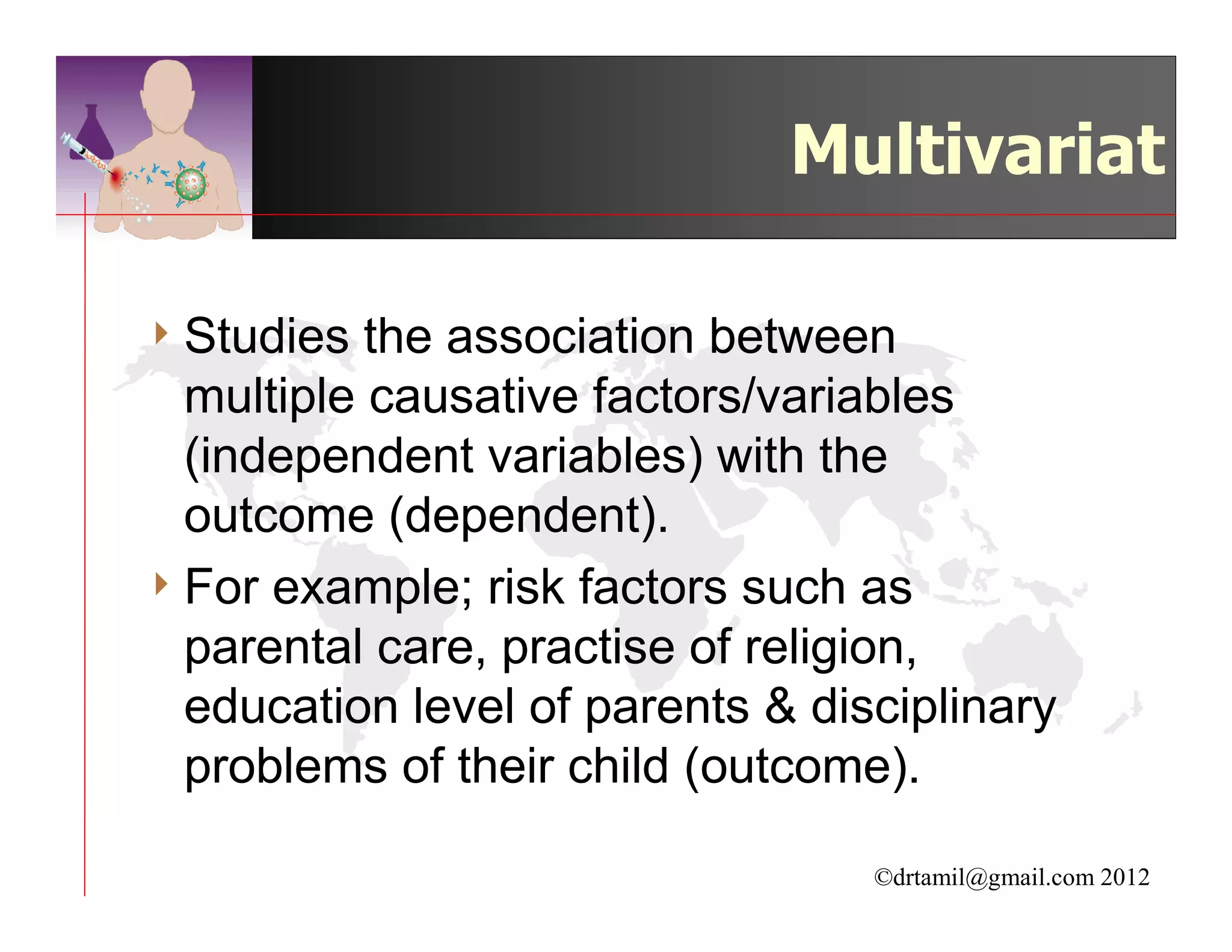
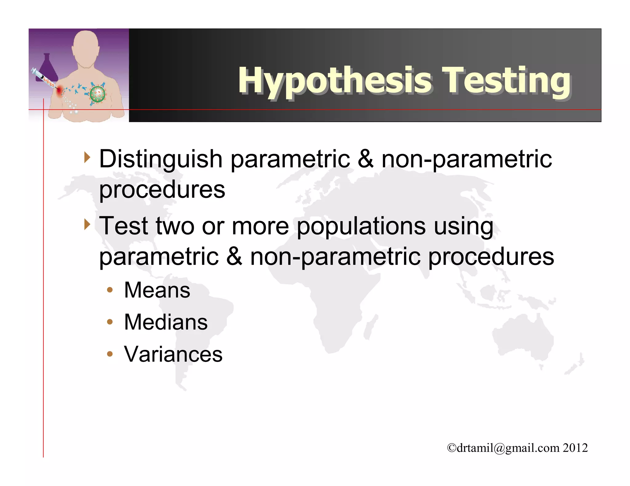
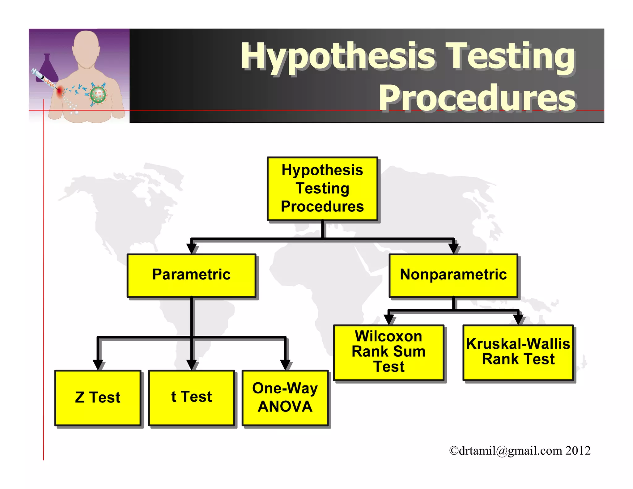
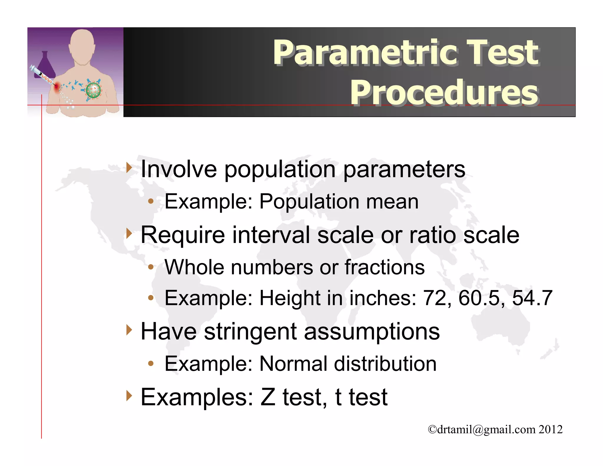
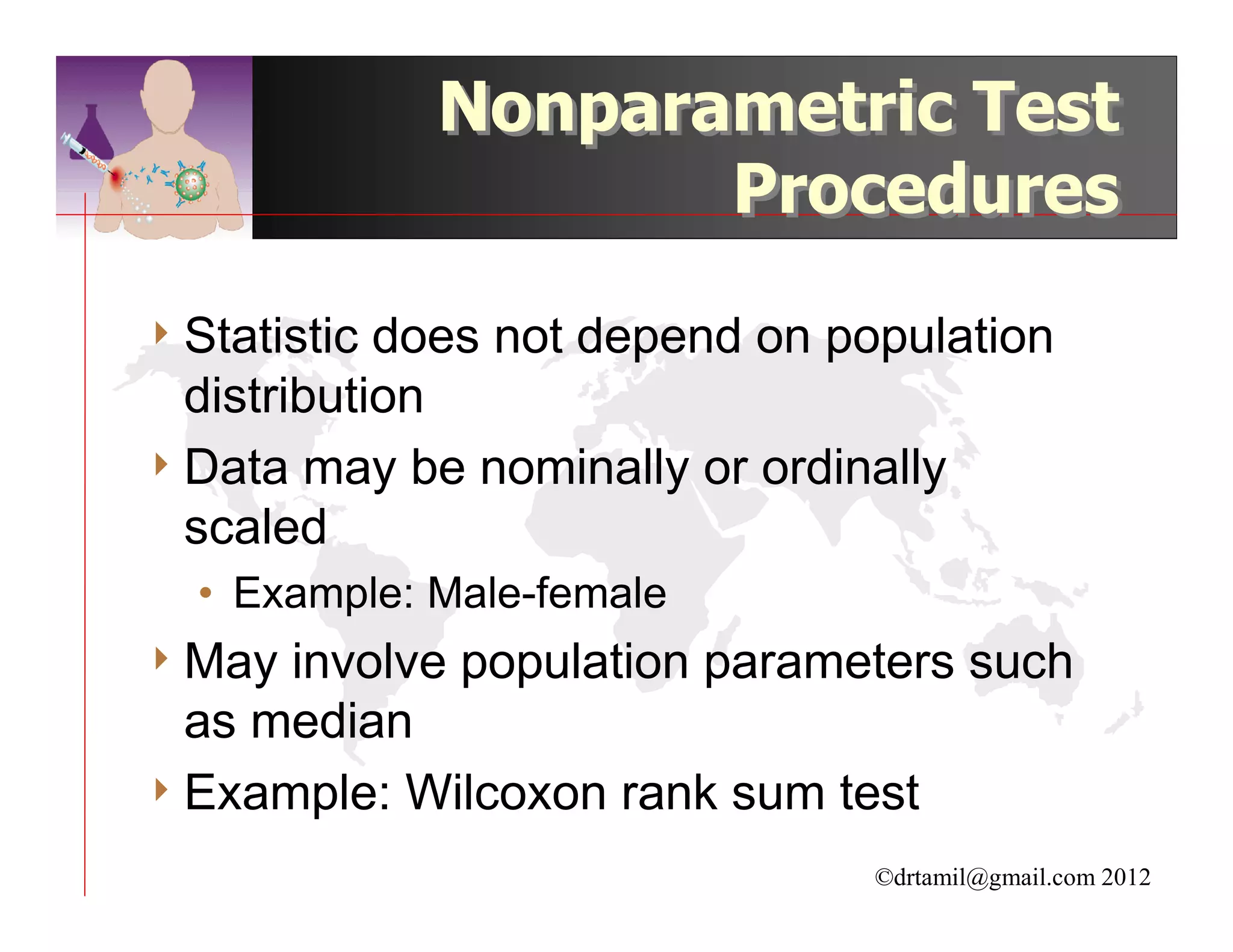
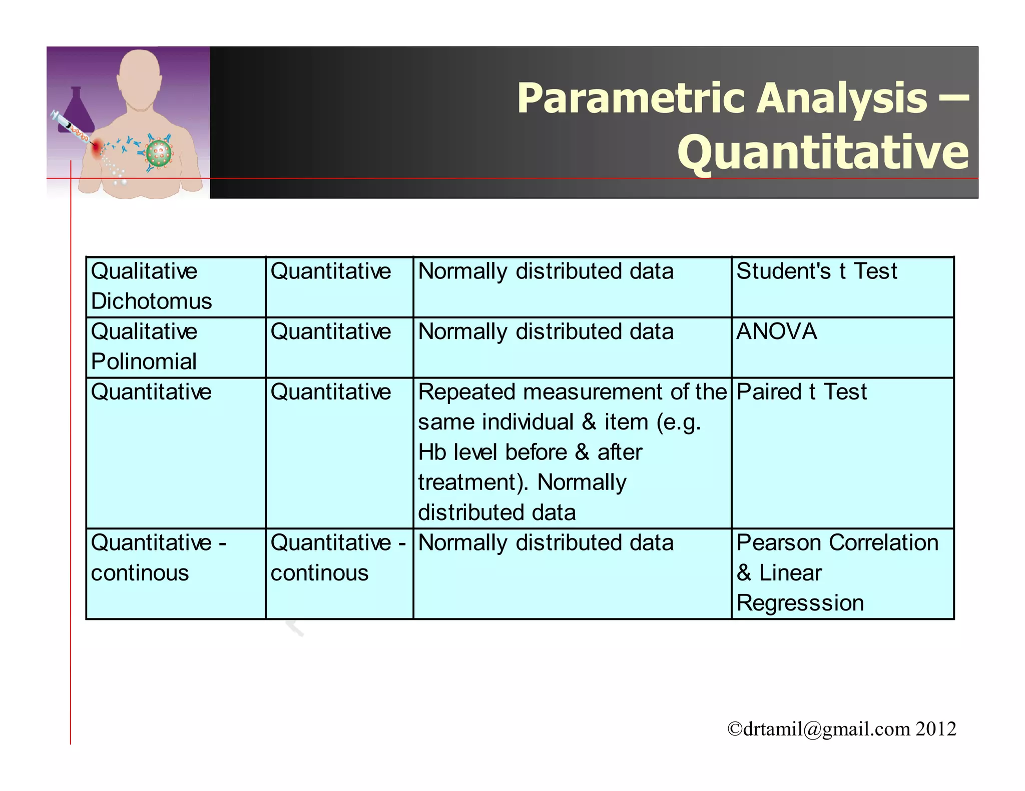
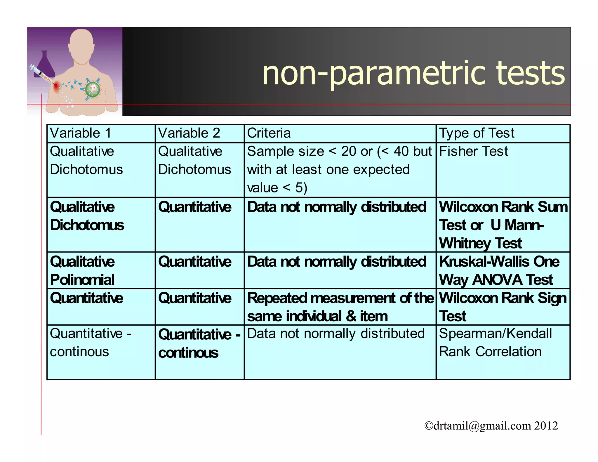
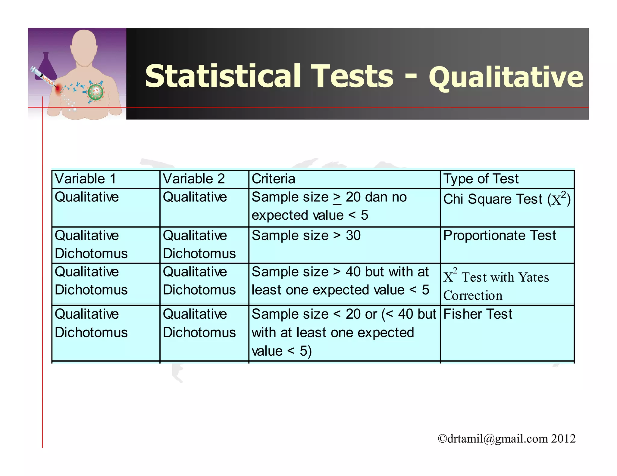
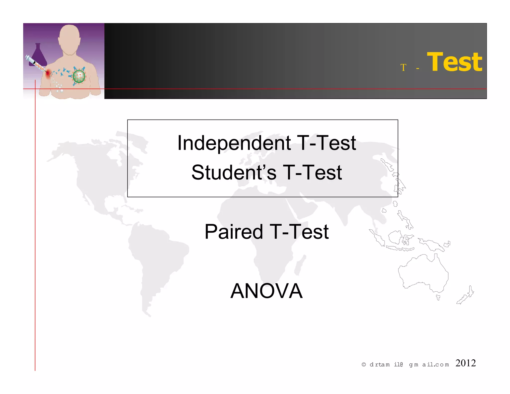
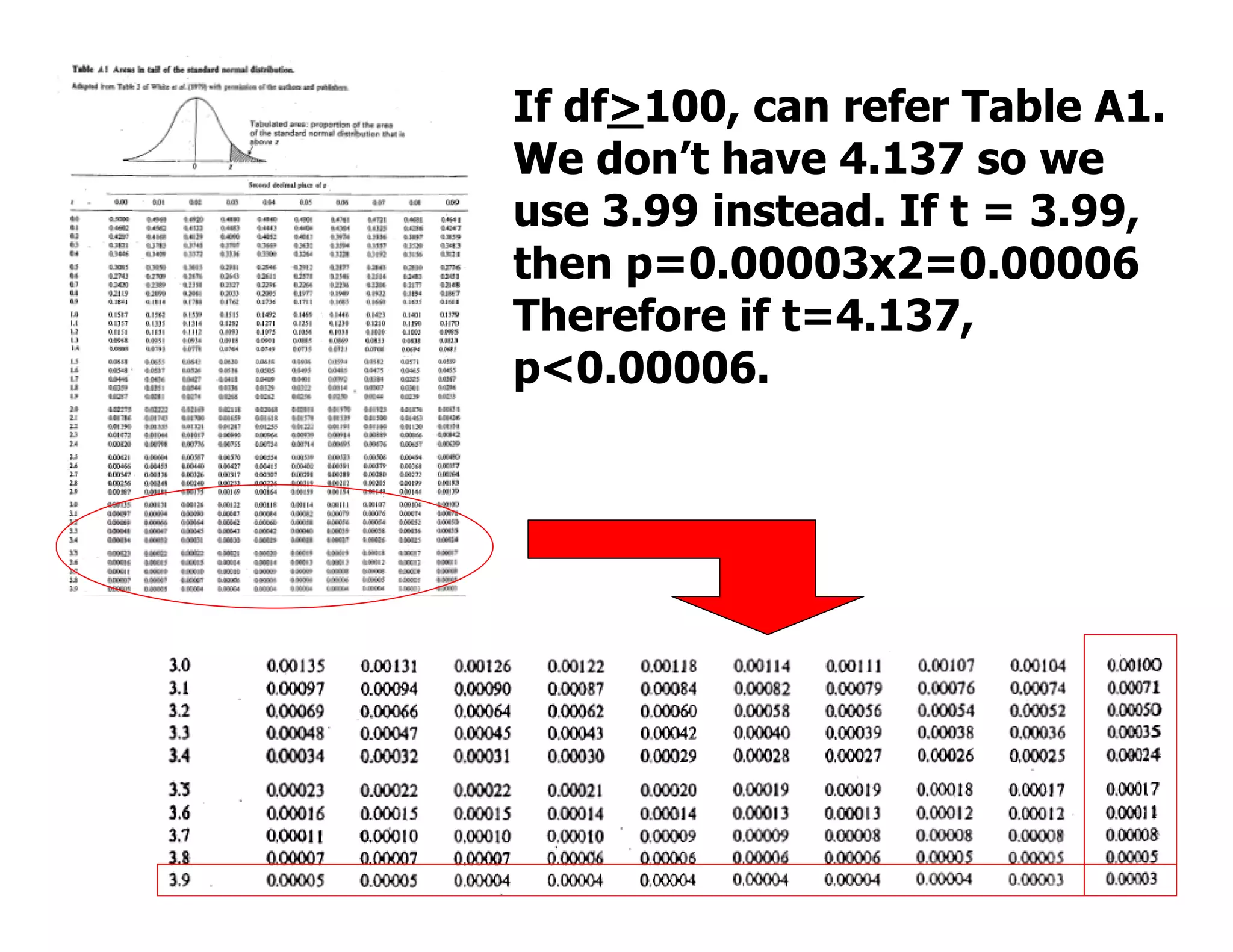
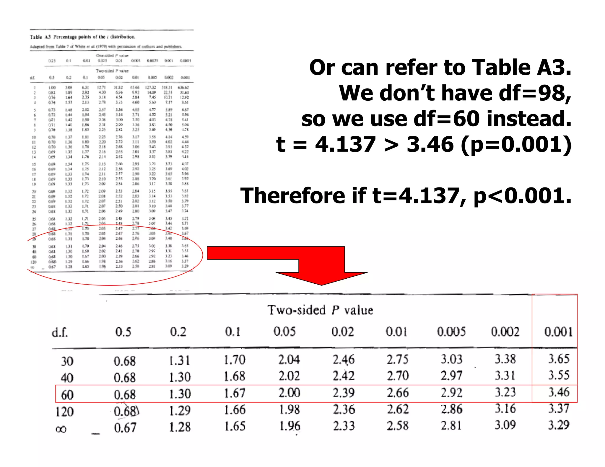
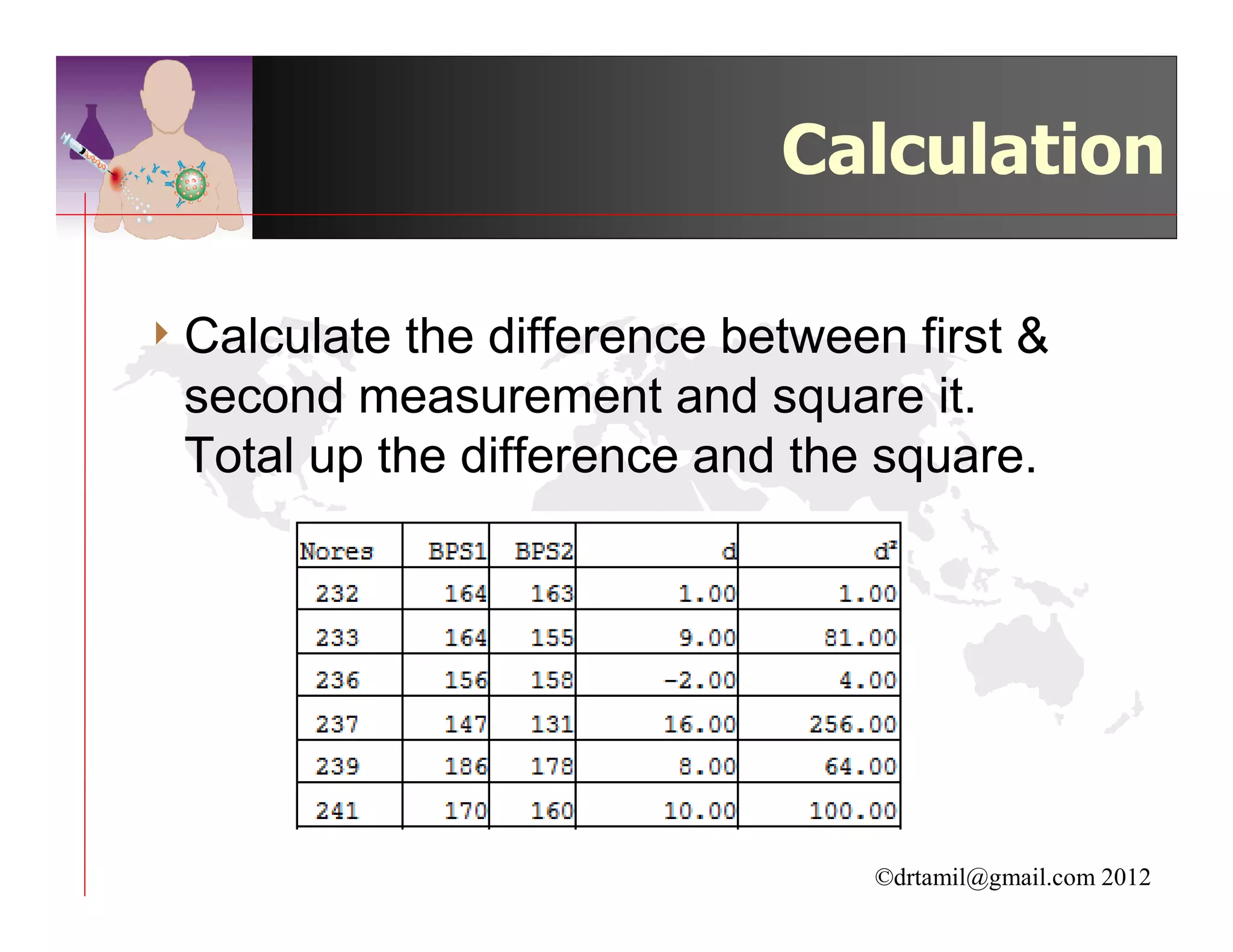
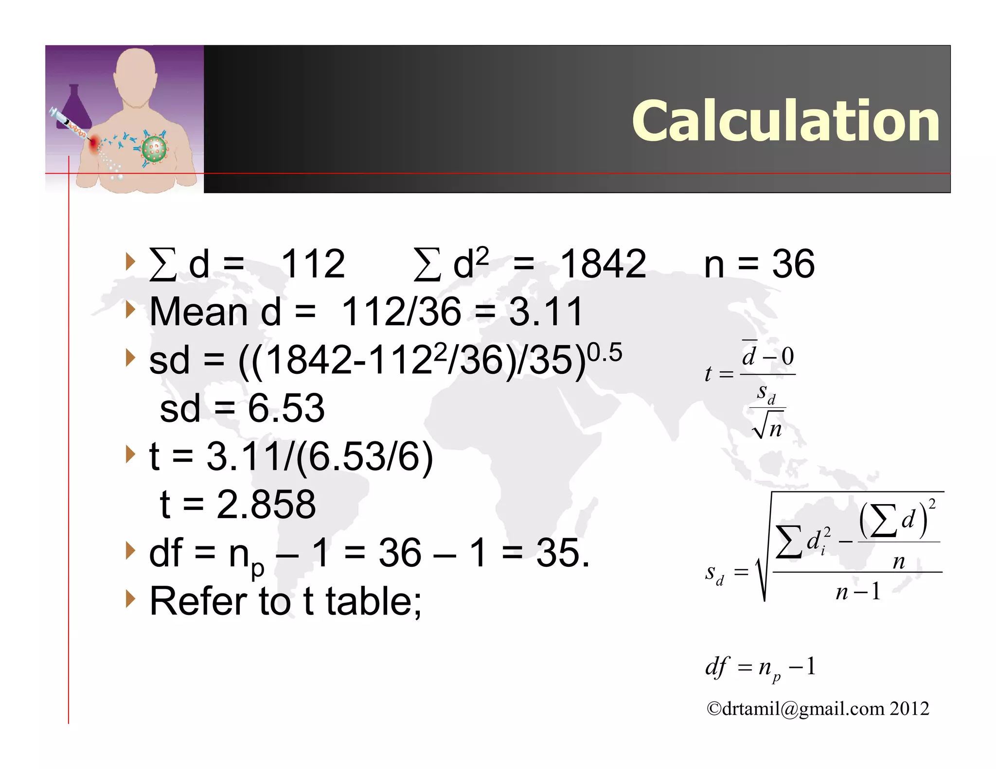
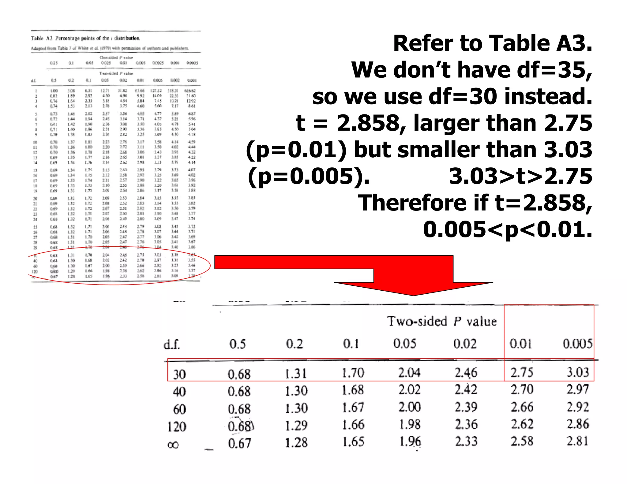
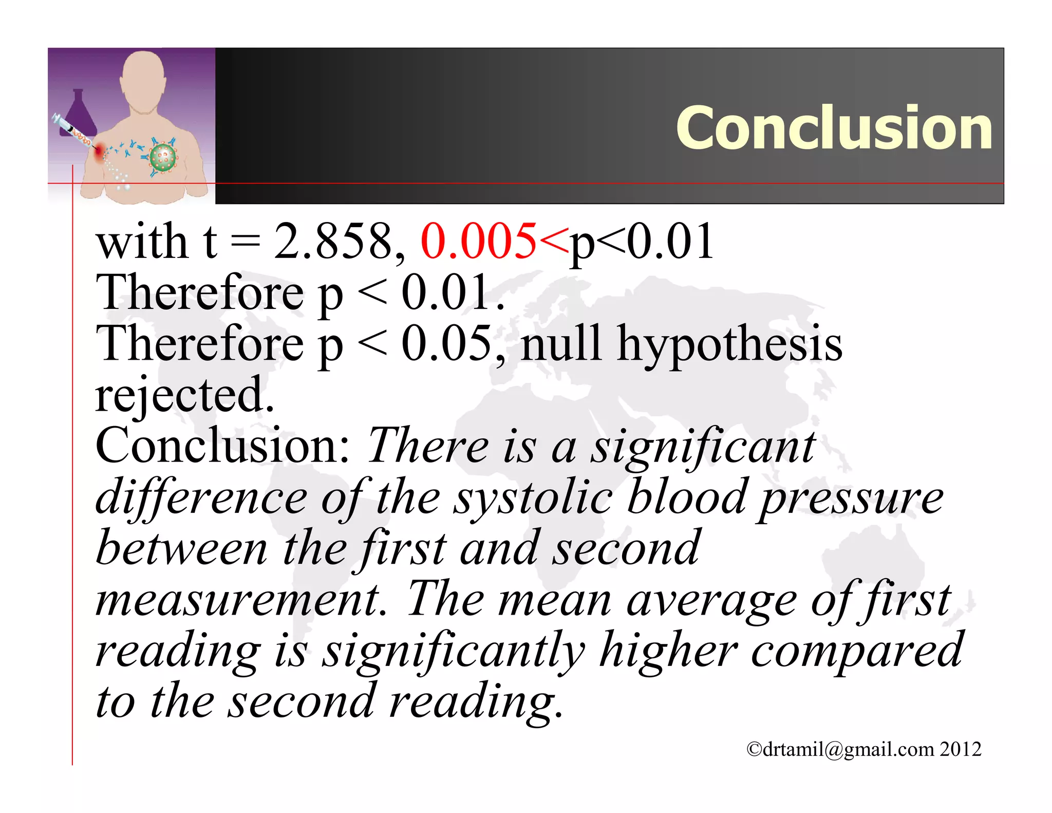
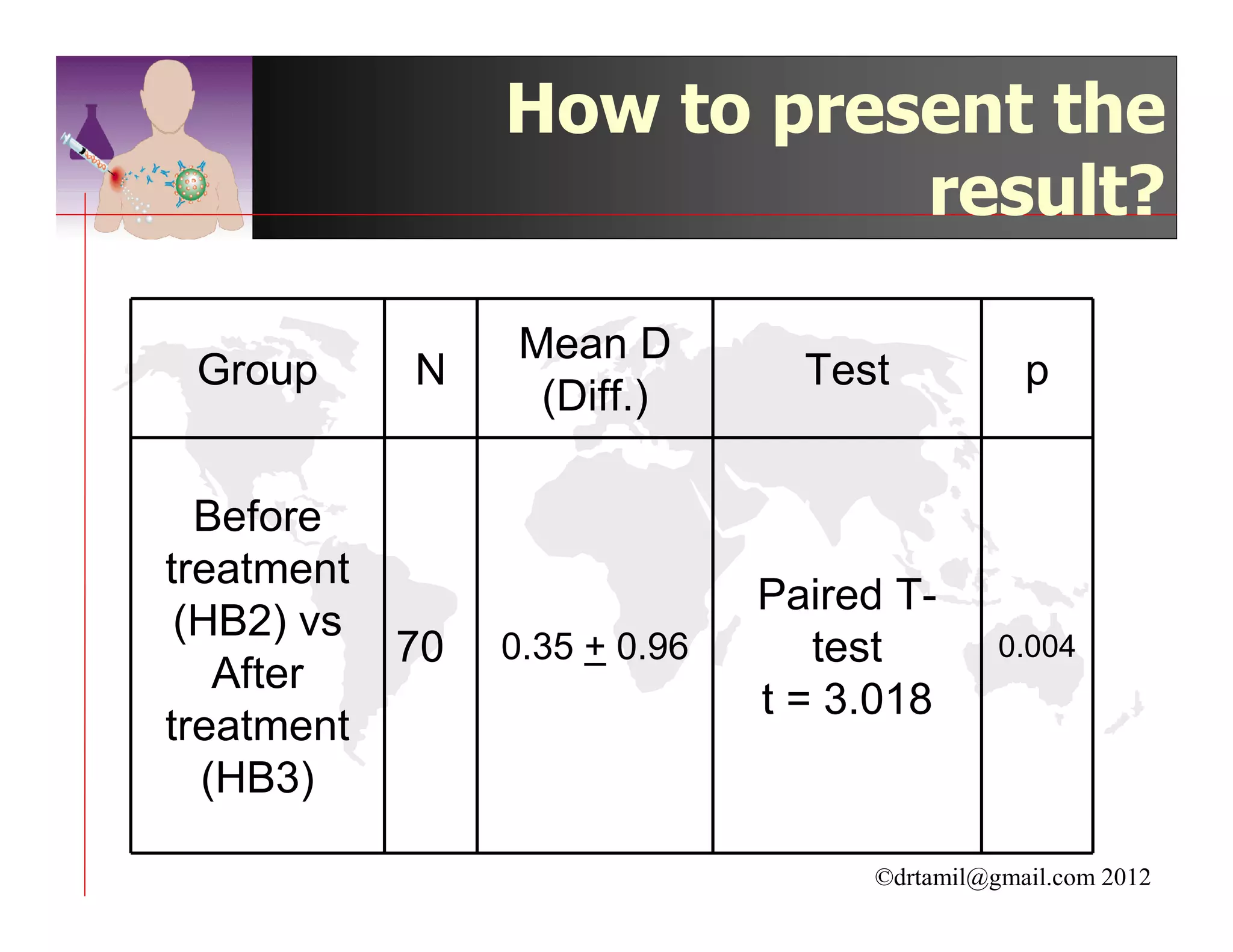


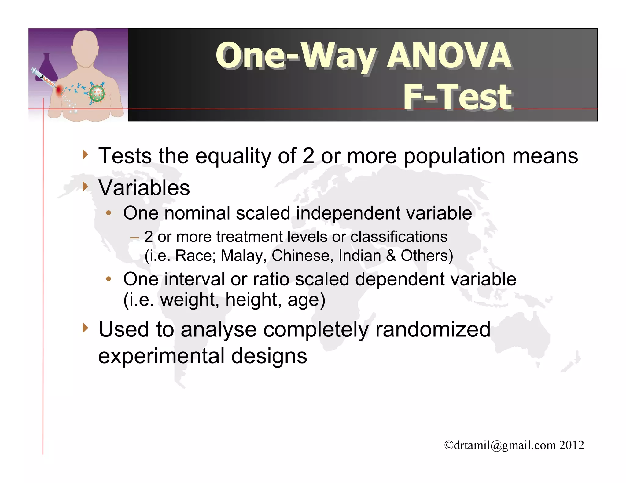
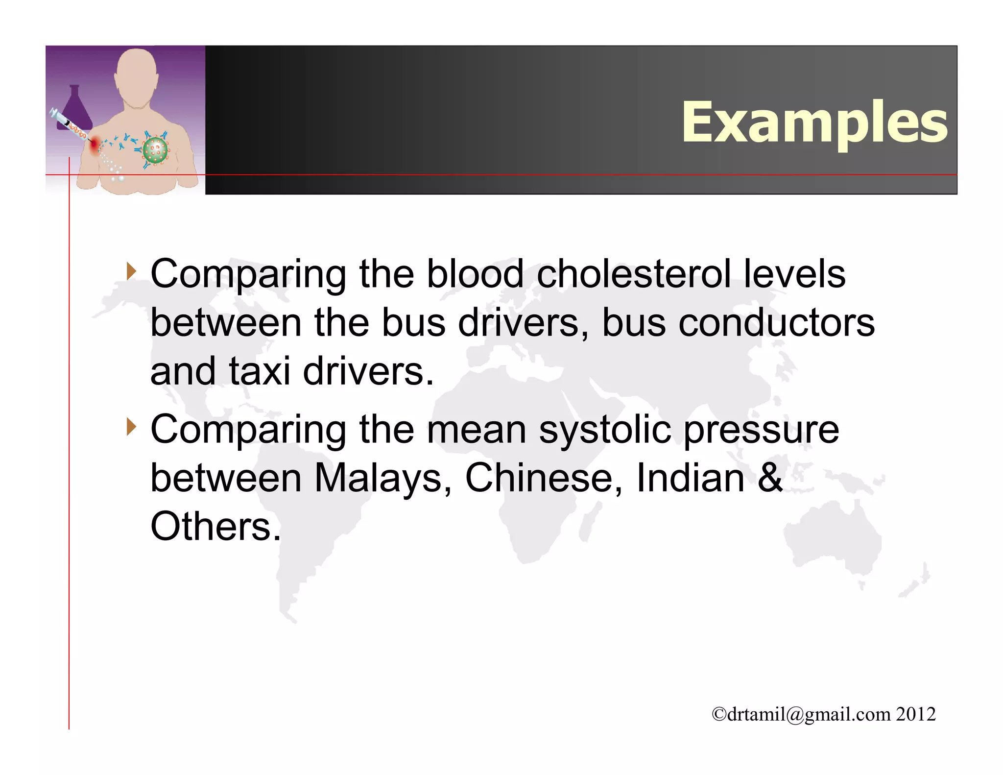

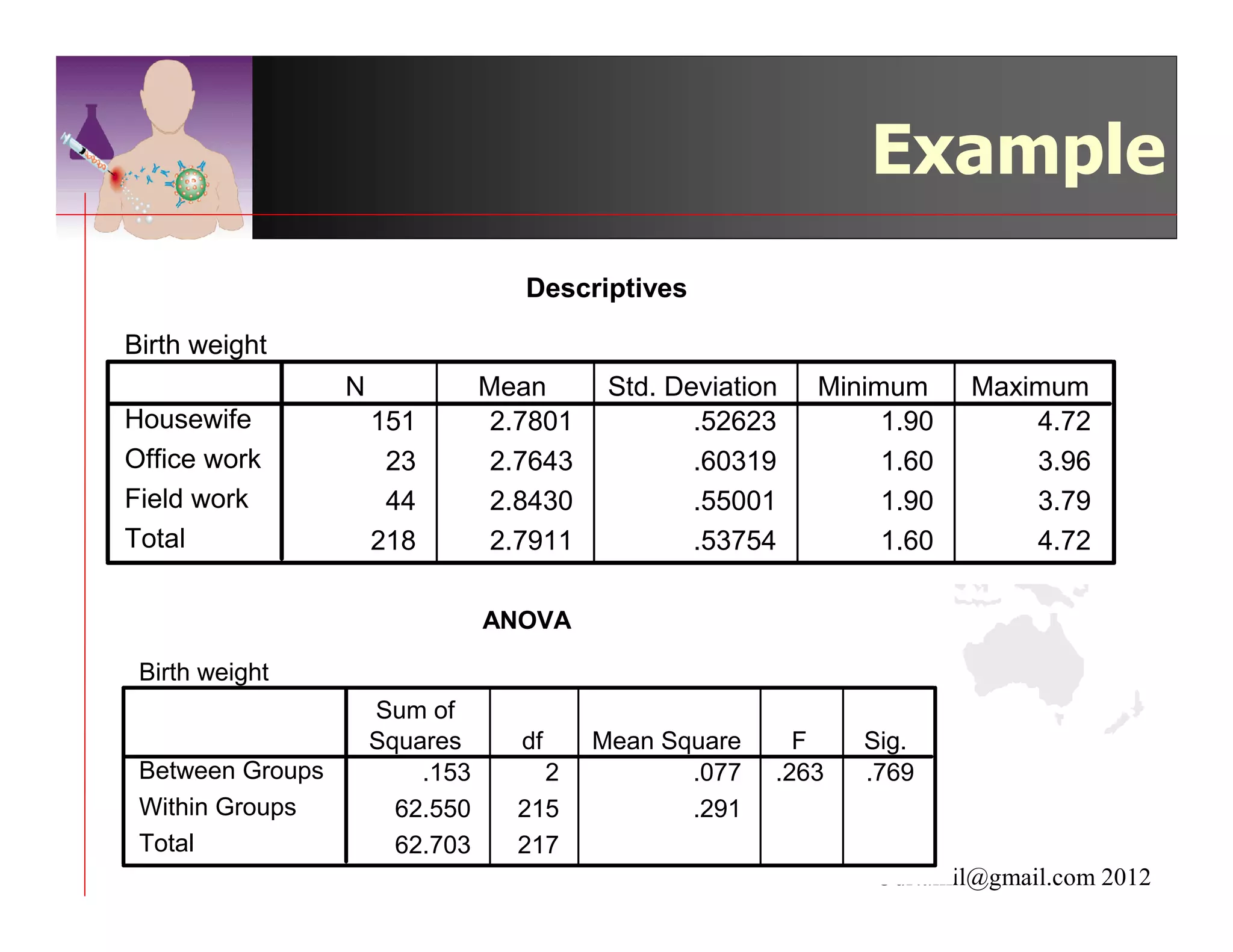
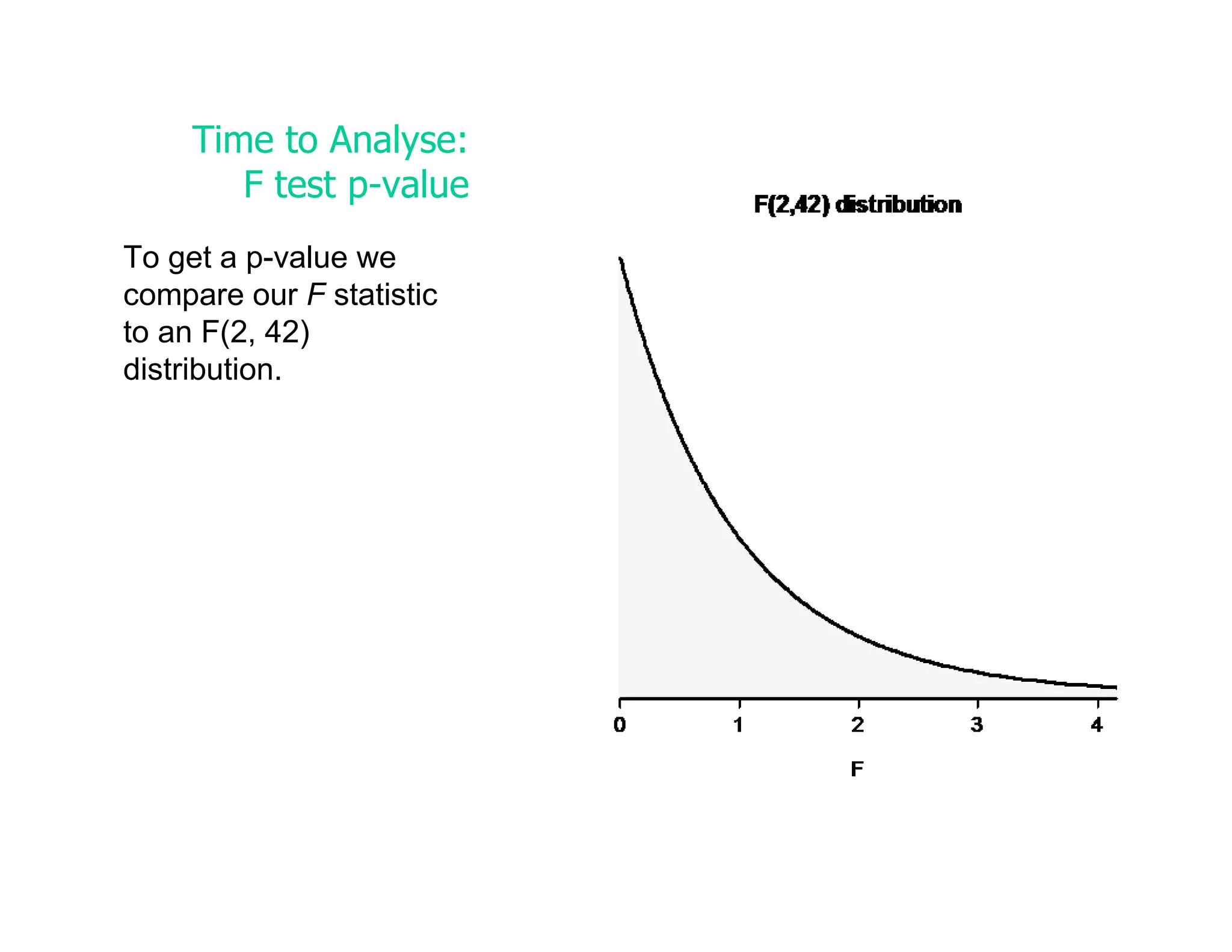

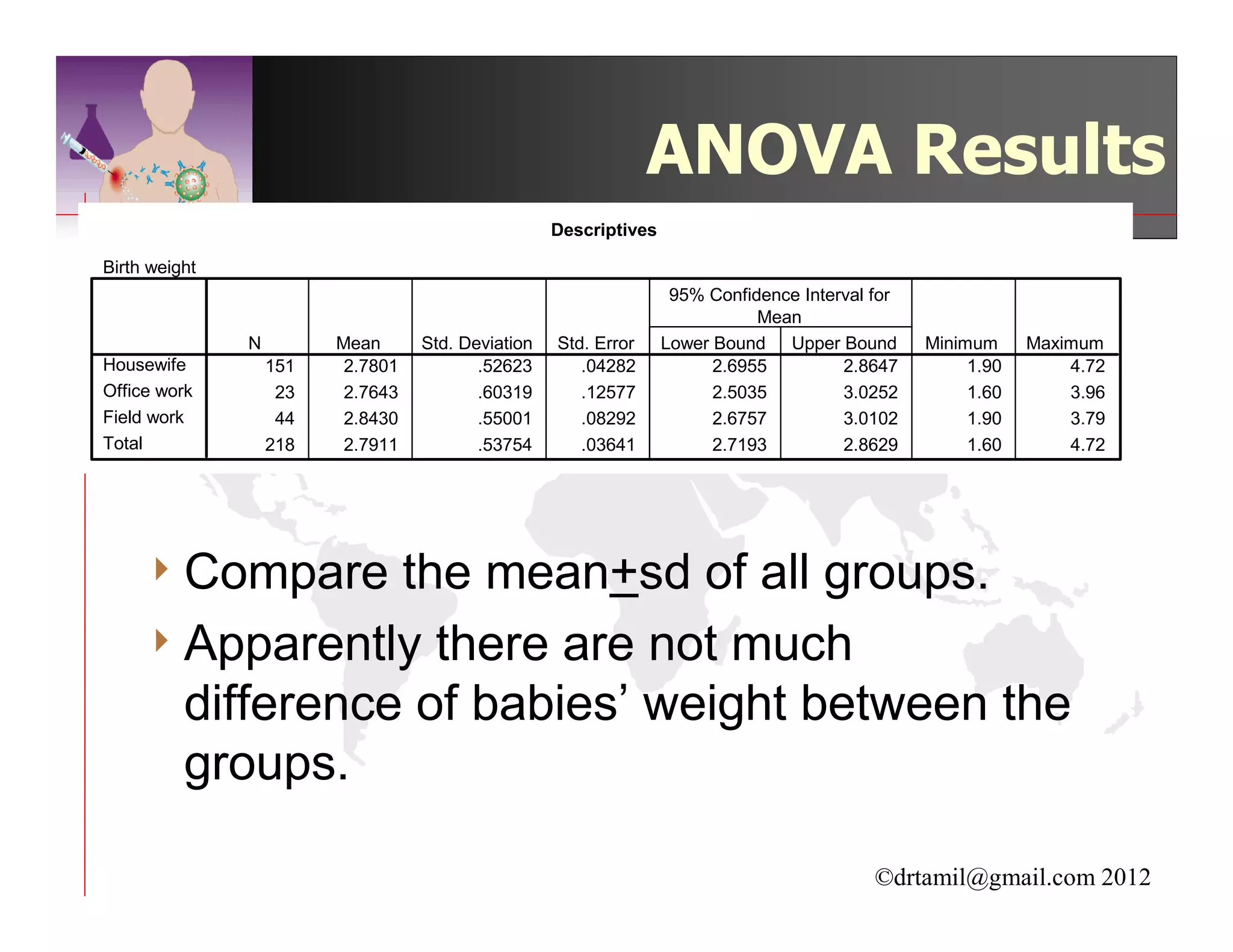
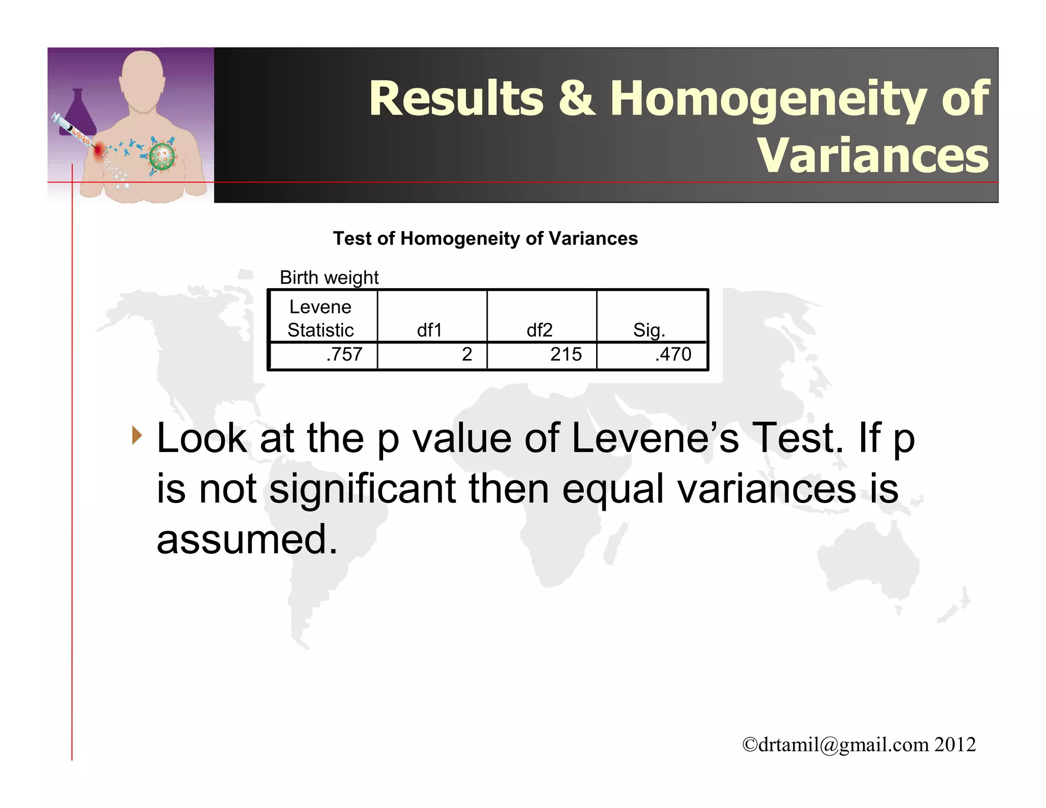
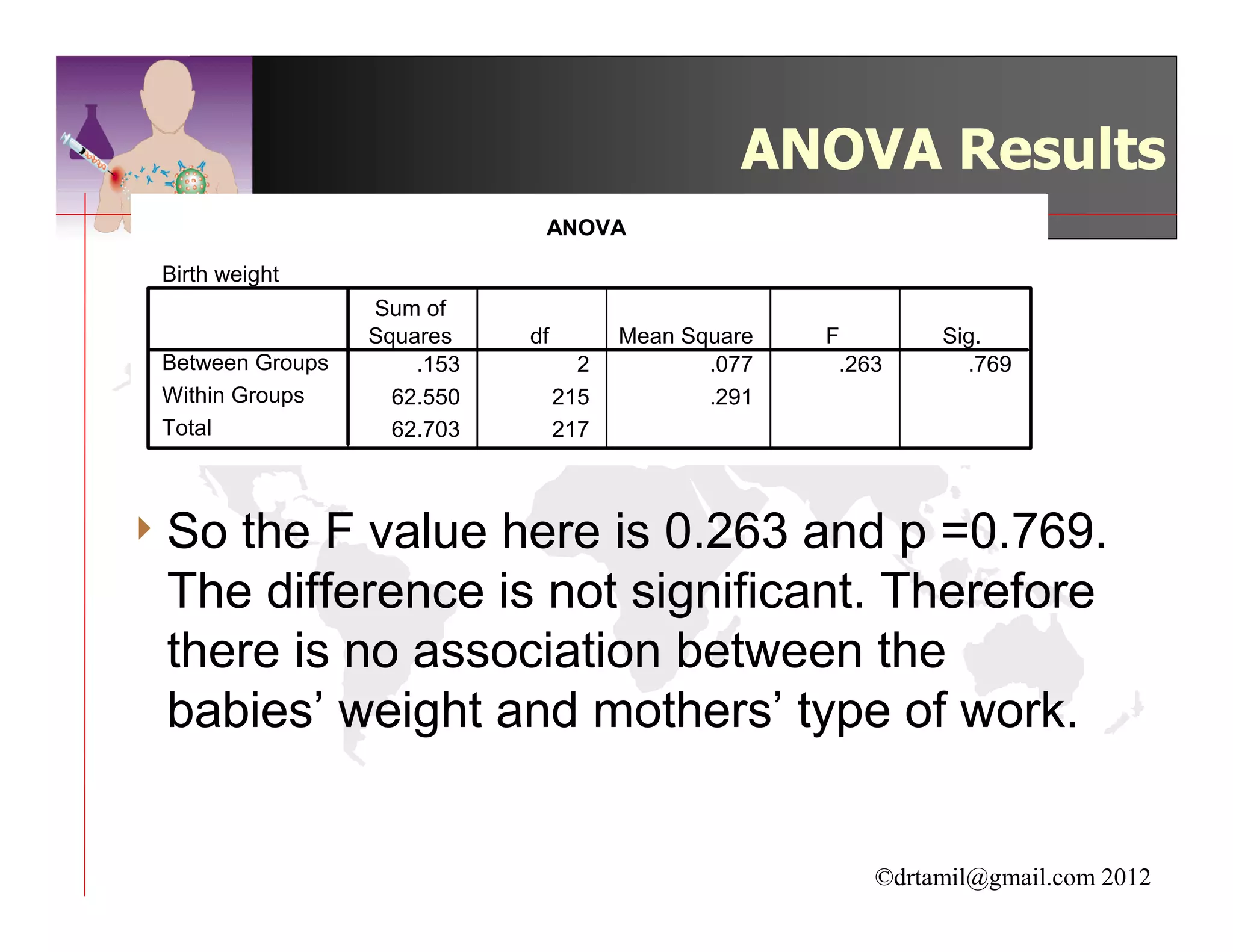
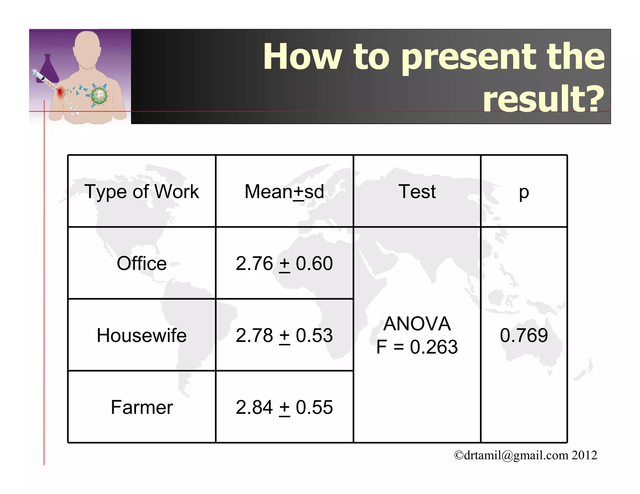
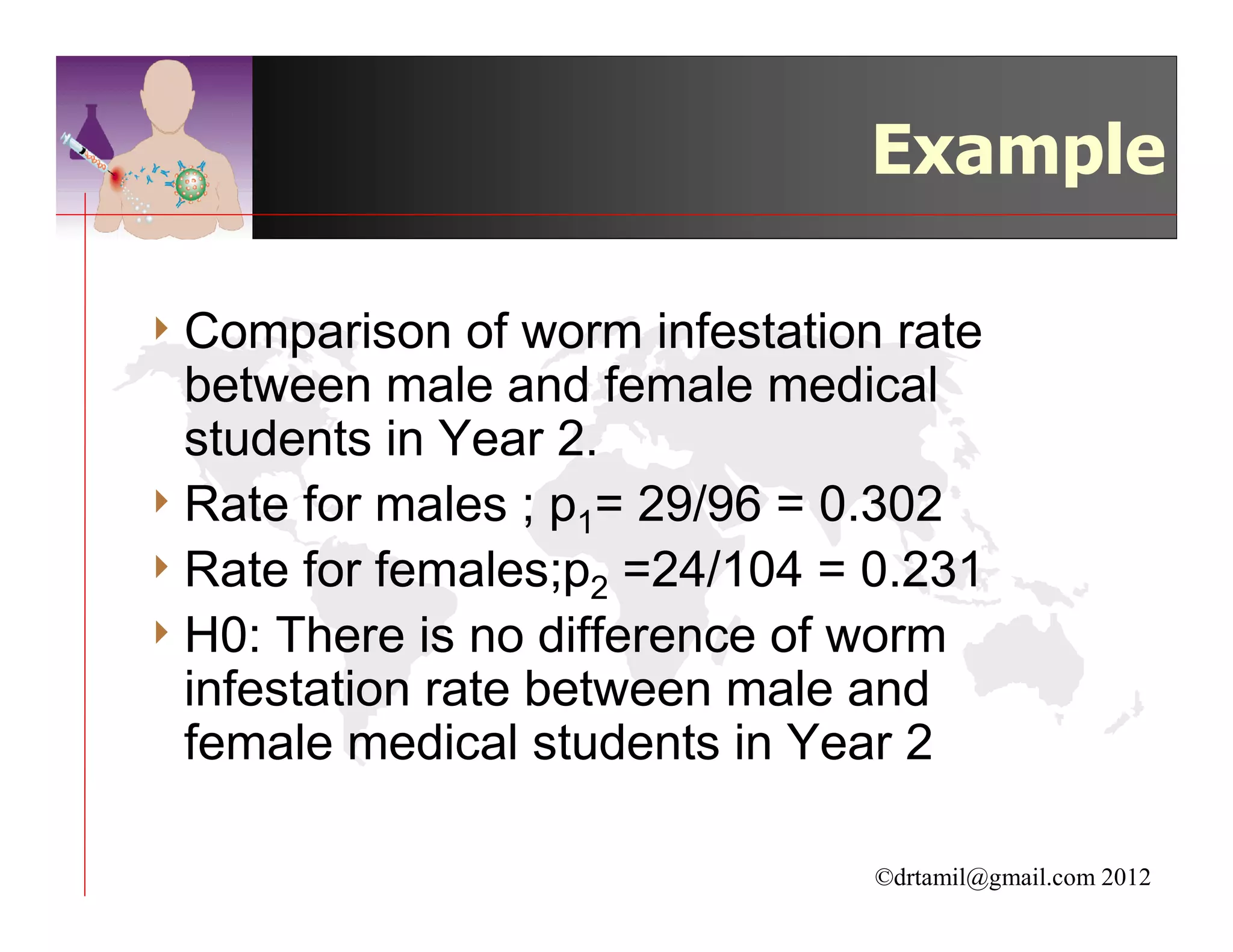
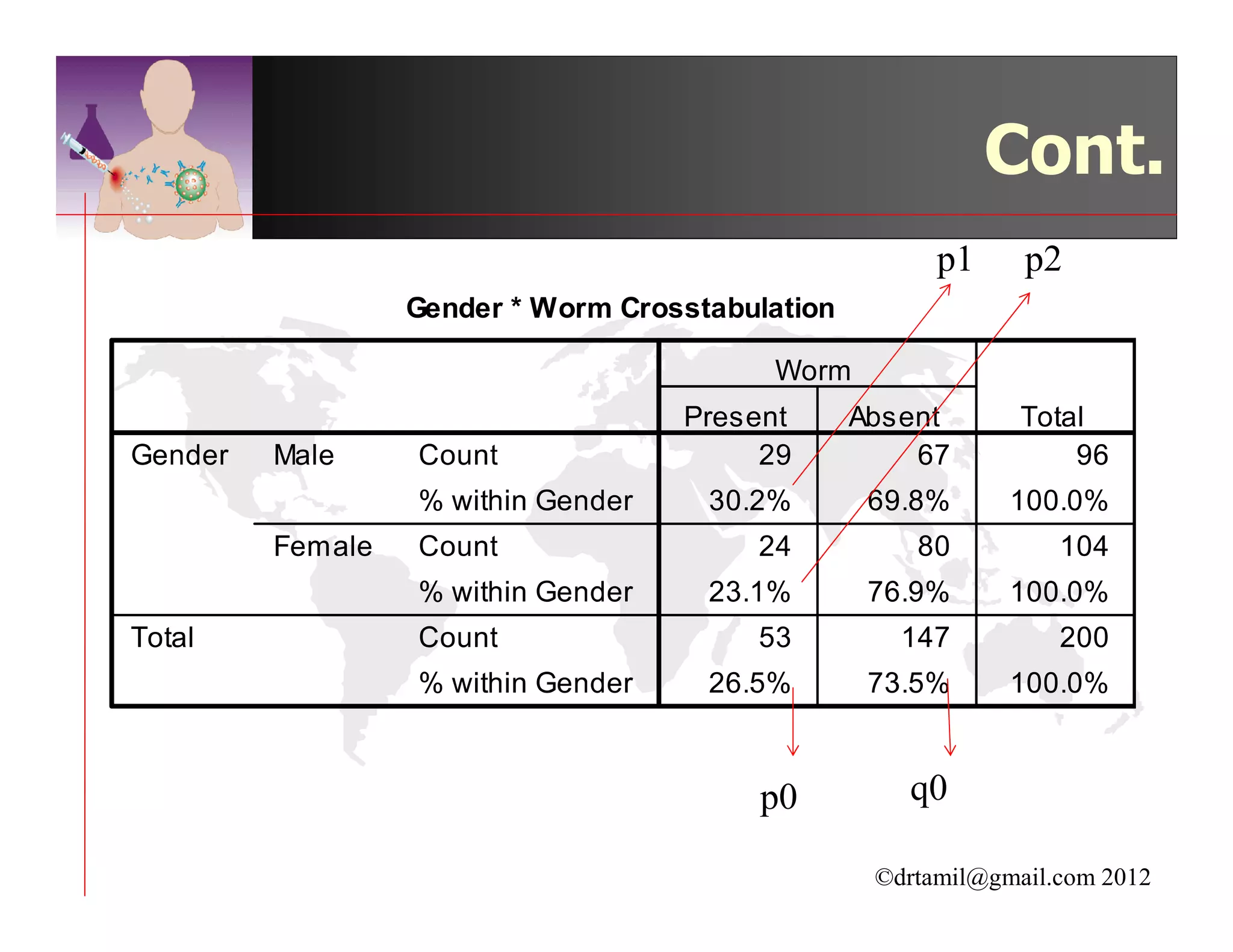
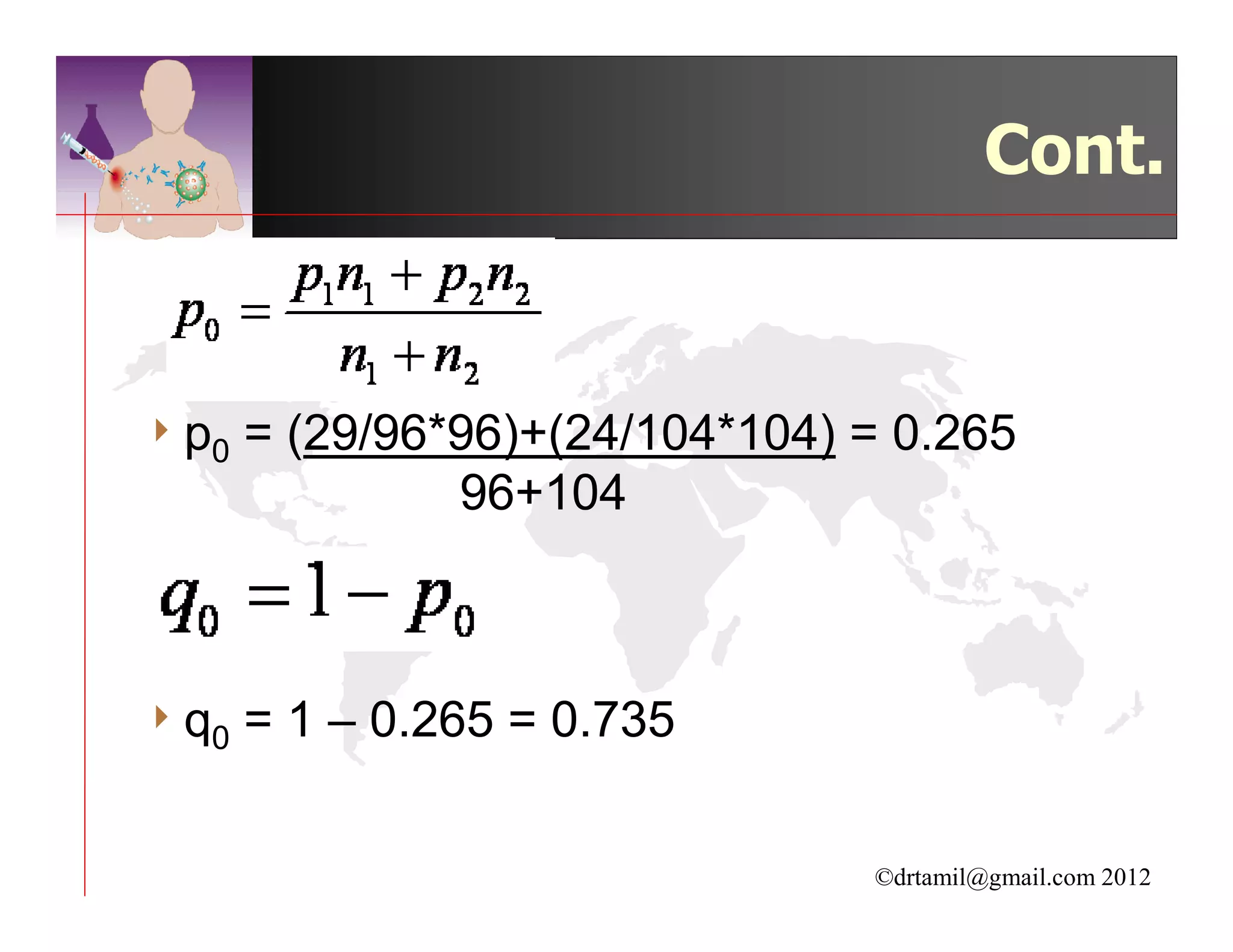
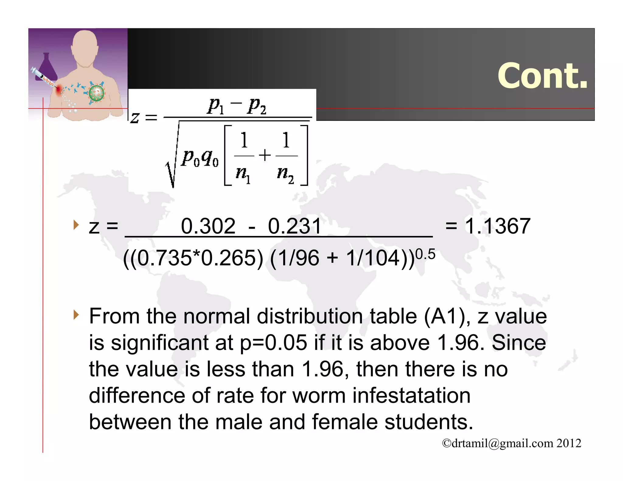

This document discusses inferential statistics and hypothesis testing. It begins by explaining the difference between descriptive and inferential statistics, and how inferential statistics are used to make inferences about populations based on data collected from samples. It then discusses key concepts in hypothesis testing including the null hypothesis, type I and type II errors, significance, confidence intervals, and p-values. Examples are provided to illustrate hypothesis testing and how to determine the appropriate statistical test to use based on the variables. Common parametric and non-parametric tests are also outlined.