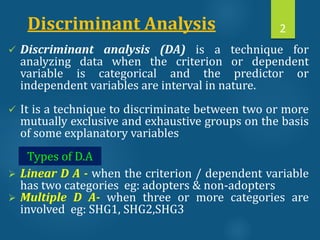
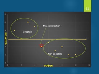
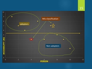
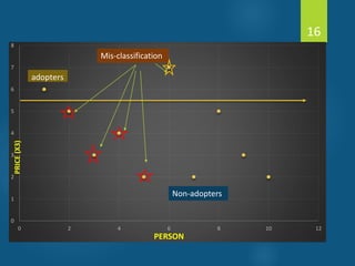
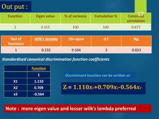
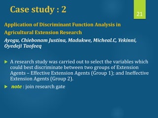
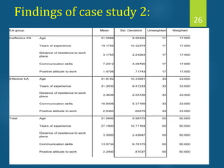
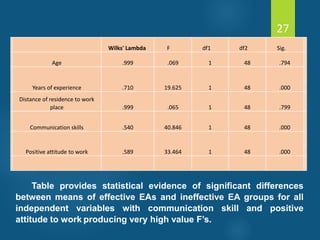
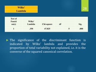
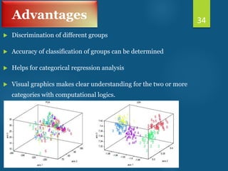
- Discriminant analysis is a statistical technique used to discriminate between two or more groups based on multiple predictor variables. - A study analyzed data on effective and ineffective extension agents to identify variables that best discriminate between the two groups. Variables like years of experience, communication skills, and positive attitude to work significantly differed between the groups. - Discriminant analysis generated a function to maximize differences between the groups based on predictor variables. The function was statistically significant based on a small Wilks' lambda value, indicating most variability was explained.

1. KRISHNA D K
ROLL NO: 20510
DIVISION OF AGRICULTURAL EXTENSION
Discriminant Analysis
1Credit Seminar

2. Discriminant Analysis
 Discriminant analysis (DA) is a technique for
analyzing data when the criterion or dependent
variable is categorical and the predictor or
independent variables are interval in nature.
 It is a technique to discriminate between two or more
mutually exclusive and exhaustive groups on the basis
of some explanatory variables
 Linear D A - when the criterion / dependent variable
has two categories eg: adopters & non-adopters
 Multiple D A- when three or more categories are
involved eg: SHG1, SHG2,SHG3
2
Types of D.A

3. Similarities and Differences
3
ANALYSIS ANOVA REGRESSION DISCRIMINANT
Similarities
1.Number of dependent One One One
variables
2.Number of independent Multiple Multiple Multiple
variables
Differences
1.Nature of the dependent Metric Metric Categorical
2.Nature of the independent Categorical Metric Metric

4. Assumptions
1. Sample size (n)
 group sizes of the dependent should not be grossly different i.e.
80:20. It should be at least five times the number of
independent variables.
2. Normal distribution
 Each of the independent variable is normally distributed.
3. Homogeneity of variances / covariances
 All variables have linear and homoscedastic relationships.
4. Outliers
 Outliers should not be present in the data. DA is highly
sensitive to the inclusion of outliers.
4

5. 5. Non-multicollinearity
 There should NOT BE MULTICOLLINEARITY among
the independent variables.
6. Mutually exclusive
 The groups must be mutually exclusive, with every
subject or case belonging to only one group.
7. Classification
 Each of the allocations for the dependent
categories in the initial classification are correctly
classified.
5

6. Discriminant Analysis Model
The discriminant analysis model involves linear combinations of
the following form:
D = b0 + b1X1 + b2X2 + b3X3 + . . . + bkXk
where
D = discriminant score
b 's = discriminant coefficient or weight
X 's = predictor or independent variable
 The coefficients, or weights (b), are estimated so that the
groups differ as much as possible on the values of the
discriminant function.
 Discriminant analysis – creates an equation which will
minimize the possibility of misclassifying cases into their
respective groups or categories
6

7. Hypothesis
 Discriminant analysis tests the following hypotheses:
H0: The group means of a set of independent variables
for two or more groups are equal.
Against
H1: The group means for two or more groups are not
equal
 This group means is referred to as a centroid.
7

8. Statistics Associated with Discriminant
Analysis
 Canonical correlation:
Canonical correlation measures the extent of association
between the discriminant scores and the groups.
 It is a measure of association between the single discriminant function and
the set of dummy variables that define the group membership.
 The canonical correlation is the multiple correlation between the
predictors and the discriminant function
 Centroid. The centroid is the mean values for the
discriminant scores for a particular group.
 There are as many centroids as there are groups, as there is
one for each group. The means for a group on all the
functions are the group centroids.
8

9.  Classification matrix. Sometimes also called
confusion or prediction matrix, the classification
matrix contains the number of correctly classified
and misclassified cases.
 Discriminant function coefficients. The
discriminant function coefficients (unstandardized)
are the multipliers of variables, when the variables
are in the original units of measurement.
 F values and their significance. These are
calculated from a one-way ANOVA, with the grouping
variable serving as the categorical independent
variable. Each predictor, in turn, serves as the metric
dependent variable in the ANOVA.
9

10.  Discriminant scores. The unstandardized
coefficients are multiplied by the values of the
variables. These products are summed and added to
the constant term to obtain the discriminant scores.
 Eigenvalue. For each discriminant function, the
Eigenvalue is the ratio of between-group to within-
group sums of squares. Large Eigenvalues imply
superior functions.
 Pooled within-group correlation matrix. The
pooled within-group correlation matrix is computed
by averaging the separate covariance matrices for all
the groups.
10

11.  Standardized discriminant function coefficients.
The standardized discriminant function coefficients
are the discriminant function coefficients and are
used as the multipliers
 Structure correlations. Also referred to as
discriminant loadings, the structure correlations
represent the simple correlations between the
predictors and the discriminant function.
 Group means and group standard deviations.
These are computed for each predictor for each
group.
11

12.  Wilks‘ lambda . Sometimes also called the U statistic,
Wilks‘ λ for each predictor is the ratio of the within-
group sum of squares to the total sum of squares. Its
value varies between 0 and 1.
 Large values of λ (near 1) indicate that group means do
not seem to be different. Small values of λ (near 0)
indicate that the group means seem to be different. It is
(1-R2 ) where R2 is the canonical correlation
 It is used to measure how well each function separates
cases into groups. It also indicates the significance of
the discriminant function and provides the
proportion of total variability not explained.
12

13. Linear discriminant analysis : Hypothetical example
Groups based on
adoption intention
quality
(x1)
accessibility
(x2)
Price
(x3)
Group A: would adopt
Person 1
Person 2
Person 3
Person 4
Person 5
8
6
10
9
4
9
7
6
4
8
6
5
3
4
2
Group B: would not
adopt
Person 6
Person 7
Person 8
Person 9
Person 10
5
3
4
2
2
4
7
5
4
2
7
2
5
3
2
13

14. 0
2
4
6
8
10
12
0 2 4 6 8 10 12
QUALITY(X1)
PERSON
adopters
14
Mis-classification
Non-adopters

15. 0
1
2
3
4
5
6
7
8
9
10
0 2 4 6 8 10 12
ACCESSIBILITTY(X2)
PERSON
adopters
15
Mis-classification
Non-adopters

16. 0
1
2
3
4
5
6
7
8
0 2 4 6 8 10 12
PRICE(X3)
PERSON
adopters
16
Mis-classification
Non-adopters

17. Out put :
Function Eigen value % of variance Cumulative % Canonical
correlation
1 3.315 100 100 0.877
17
Test of
functions
Wilk’s lambda Chi-squre d.f. Sig.
1 0.232 9.504 3 0.023
Function
1
X1 1.110
X2 0.709
x3 -0.564
Standardised canonical discrimination function coefficients
Zi = 1.110x1+0.709x2-0.564x3
Discriminant function can be written as
Note : more eigen value and lesser wilk’s lambda preferred

18. Predicting group membership:
 Group centroids are calculated as 10.77 and 4.52.
by taking the mean of respective discriminant
scores of the Group. Thus the cut of score is
average of both = 7.65
 One can predict a person’s choice of dependent
variable i.e. adopting / non – adopting
18

19. Multiple discriminant analysis
 When we need to discriminate among more
than two groups, we use multiple
discriminant analysis.
 This technique requires fitting g-1 number of
discriminant functions, where g is the
number of groups
 Assumptions remain same for this type too..
 The best D will be judged as per the
comparison between functions
19

20. Case study 1:
Title : A study on agri-entrepreneurship behaviour of farmers
author : Dipika hajong (2014)
tool used for : to discriminate between variables which contribute for
behaviour in agripreneurs and non-agripreneurs
Sample size : 20 entrepreneurs and 30 conventional farmers
Variables : aspiration, information processing behaviour, proactiveness,
information passing frequency , social network , resiliency , autonomy,
total land & hope of success
Finding : confidential
20

21. Case study : 2 21
Application of Discriminant Function Analysis in
Agricultural Extension Research
Ayogu, Chiebonam Justina, Madukwe, Micheal.C, Yekinni,
Oyedeji Taofeeq
 A research study was carried out to select the variables which
could best discriminate between two groups of Extension
Agents – Effective Extension Agents (Group 1); and Ineffective
Extension Agents (Group 2).
 note : join research gate

22. 1. Analyse ˃>>Classify >>>Discriminant 22

23. 2. Click Define Range button and enter
the lowest and highest code for your
groups.
23

24. 243.Click on Statistics button and select Means, Univariate
Anovas, Box’s M,

25. 254. Click on Save and then select Predicted Group
Membership and Discriminant Scores, click Continue

26. Findings of case study 2:
26
EA group Mean Std. Deviation Unweighted Weighted
Ineffective EA Age 31.0588 8.20420 17 17.000
Years of experience 19.1765 10.42374 17 17.000
Distance of residence to work
3.1765 2.24264 17 17.000
place
Communication skills 7.2312 4.28795 17 17.000
Positive attitude to work 1.4706 .71743 17 17.000
Effective EA Age 31.8182 10.33941 33 33.000
Years of experience 31.3030 8.47233 33 33.000
Distance of residence to work
3.3636 2.54728 33 33.000
place
Communication skills 16.8406 5.37169 33 33.000
Positive attitude to work 2.6364 .65279 33 33.000
Total Age 31.5600 9.58775 50 50.000
Years of experience 27.1800 10.77164 50 50.000
Distance of residence to work
3.3000 2.42647 50 50.000
place
Communication skills 13.5734 6.78175 50 50.000
Positive attitude to work 2.2400 .87037 50 50.000

27. Wilks' Lambda F df1 df2 Sig.
Age .999 .069 1 48 .794
Years of experience .710 19.625 1 48 .000
Distance of residence to work
place .999 .065 1 48 .799
Communication skills .540 40.846 1 48 .000
Positive attitude to work .589 33.464 1 48 .000
27
Table provides statistical evidence of significant differences
between means of effective EAs and ineffective EA groups for all
independent variables with communication skill and positive
attitude to work producing very high value F’s.

28. 28
Test of
Functi Wilks'
on(s) Lambda Chi-square df Sig.
1 .350 47.825 5 .000
Wilks'
Lambda
 The significance of the discriminant function is
indicated by Wilks’ lambda and provides the
proportion of total variability not explained, i.e. it is the
converse of the squared canonical correlation.

29. Pooled Within-Groups Matrices
Distance of Positive
Years of residence to Communicatio attitude to
Correlation age experience work place n skills work
Age 1.000 .094 -.149 -.036 .243
Years of experience .094 1.000 -.231 .139 .021
Distance of residence
-.149 -.231 1.000 -.198 -.303
to work place
Communication skills -.036 .139 -.198 1.000 .214
Positive attitude to work
.243 .021 -.303 .214 1.000
29
The within- groups correlation matrix shows the correlations
between the predictors.

30. 30
An eigenvalue provides information on the proportion of
variance explained. A canonical correlation of 0.807 suggests the
model explains 65.13% (i.e.0.8072 ×100) of the variation in the
grouping variable, i.e. whether an extension agent is effective or
ineffective
Eigenvalues table
Functi Canonical
on Eigenvalue % of Variance Cumulative % Correlation
1 1.861a
100.0 100.0 .807

31. Structure matrix table 31
Function
1
Communication skills .676
Positive attitude to work .612
Years of experience .469
age .028
Distance of residence to work
.027
place
These unstandardized coefficients (b) operate like unstandardized b
(in regression) coefficients and are used to create the actual
prediction equation which are used to classify new cases.

32. 32
Canonical Discriminant Function Coefficients table
Age
Years of experience
Distance of residence to
work place
Communication skills
Positive attitude to work
(Constant)
Unstandardized coefficients
Function
1
-.009
.053
.175
.110
.940
-5.329

33.  D= (-0.009 age) + (0.053 × years of experience in
extension work) + (0.175 × distance of residence to work
place) + (0.110 × communication skill) + (0.940 ×
positive attitude to work) - 5.329.
33

34. Advantages
 Discrimination of different groups
 Accuracy of classification of groups can be determined
 Helps for categorical regression analysis
 Visual graphics makes clear understanding for the two or more
categories with computational logics.
34

35.  Linear discrimination cannot be used when
subgroups are stronger.
 The selection of the predictor variables are not
strong until a strong classification exists.
 It cannot be used when there is insufficient data to
define sample means
35
Limitations

36. Contd…
 If the number of observations are less, the discrimination
method cannot be used.(5 times more than the no. of
predictor variables) : Lawrence – applied
multivariate research)
 If the overlap in the distribution is small, the discriminant
function separates the groups well.
 If the overlap is large, the function is a poor discriminator
between the groups.
36

37. Applications
Prediction and description DA (Lawrence : applied multivariate research)
Agriculture- Fisheries, Crop studies, yield studies, Geoinformatics, Bioinformatics, social science
researches
Socio-economics and Behavioral studies of rural communities
Hydrological and physico-chemical studies in different water resources
Bankruptcy prediction based on accounting ratios and other financial variables (LDA)
Face recognition (Computerized)
Marketing –Different types of customers and products based on surveys.
37

38. References
1. Hajong Dipika.(2014). A study on agri-entrepreneurship
behaviour of farmers. PhD thesis. IARI, New Delhi
2. Kothari, C. R. (2004). Research methodology: Methods and
techniques. New Age International.
3. Meyers, L. S., Gamst, G., & Guarino, A. J. (2006). Applied
multivariate research: Design and interpretation. Sage.
4. Poulsen, J., & French, A. (2008). Discriminant function
analysis. San Francisco State University: San Francisco, CA.
5. SPSS Chapter 25 Data File B. Retrieved from
www.uk.sagepub.com/
6. www.youtube.com/watch?v=7zYcMZ-61c4
38

39. 39