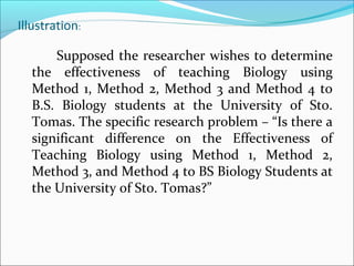
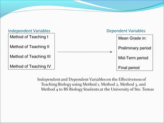
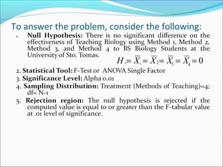
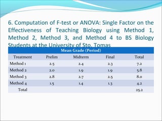
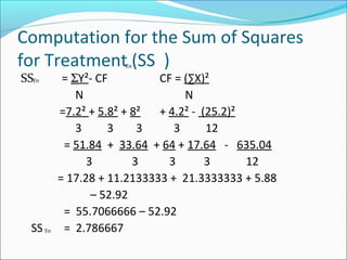
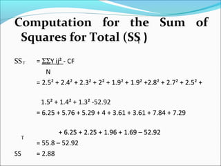
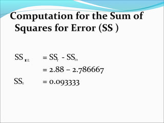
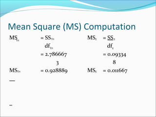
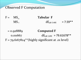
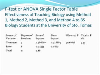
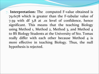
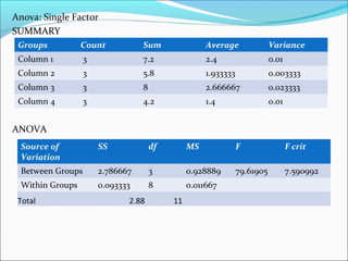
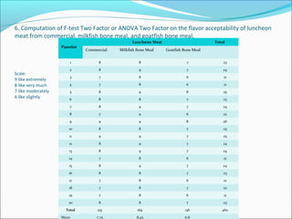
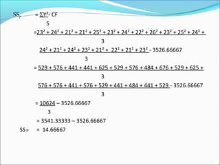
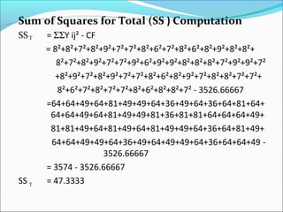
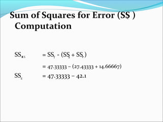
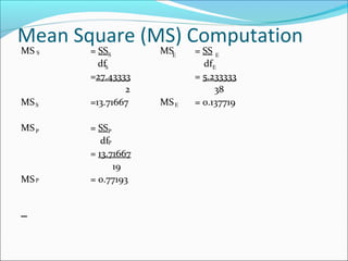
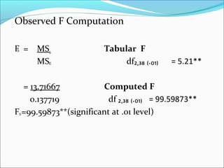
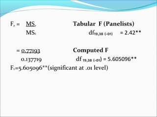
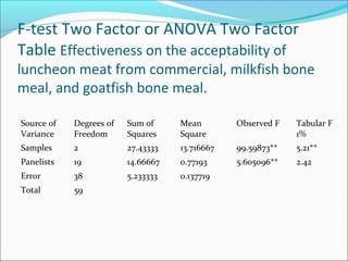
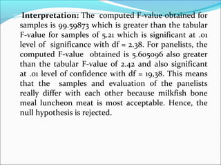
ANOVA analysis was conducted to compare the effectiveness of 4 teaching methods on student grades. The analysis found a significant difference between the methods (F=79.61678, p<0.01), with Method 4 being most effective. A second ANOVA compared acceptability of luncheon meat from 3 sources using 20 panelists, finding significant differences between sources (F=99.59873, p<0.01) and panelists (F=5.605096, p<0.01).

1. Prepared by:
MARIANNE G. MALUYO

2. F-Test or Analysis of Variance
(ANOVA)
- An inferential statistics used to
determine the significant
difference of three or more
variables or multivariate
collected from experimental
research.

3. F-test: single factor analysis of
variance involves the
independent variables as basis
for classification. This is usually
applied in single-group design
and complete randomized
design (CRD).

4. Step 1. Partition the sum of
squares for treatment,
error, and total by using
the appropriate formula:

5. Computation for the Sum of
Squares for Treatment (SS )
SS = ΣY²- CF
N
Where:
SS = Sum of squares for treatment
ΣY² = Sum of squared total for treatment
CF = Correction factor or CF = (ΣX)²
N
rtΤ
rtΤ
rtΤ

6. Computation for the Sum of
Squares for Total (SS )
SS = ΣΣYij² - CF
N
Where:
SS = Sum of squares for treatment
ΣΣYij = Sum of squared total for treatment
CF = Correction factor
Τ
T
Τ

7. Computation for the Sum of
Squares for Error (SS )
SS = SS - SS
Ε
Ε Τ rtΤ

8. Step 2. Divide the sum of squares
for treatment, error, and total
with the corresponding degrees of
freedom (df), df=N-1, to get the
mean square by using this
formula, MS=SS/df

9. Step 3. Divide the mean square treatment by
mean square to get the F-value. The
formula in getting F equals mean square
for treatment
(MS ) divided by mean square for error
(MS ) which is expressed as follows:
F= MS
MS
rtΤ
rtΤ
Ε
Ε

10. Step 4. Refer to the F –distribution
table in the appendix to determine
if the computed F value is
significant or not at .01 or .05 level
of confidence

11. Step 5. Prepare F-test or ANOVA
Table by entering the values of
Steps 1, 2 and 3.

12. Illustration:
Supposed the researcher wishes to determine
the effectiveness of teaching Biology using
Method 1, Method 2, Method 3 and Method 4 to
B.S. Biology students at the University of Sto.
Tomas. The specific research problem – “Is there a
significant difference on the Effectiveness of
Teaching Biology using Method 1, Method 2,
Method 3, and Method 4 to BS Biology Students at
the University of Sto. Tomas?”

13. Independent Variables Dependent Variables
Method of Teaching I
Method of Teaching II
Method of Teaching III
Method of Teaching IV
Mean Grade in:
Preliminary period
Mid-Term period
Final period

14. To answer the problem, consider the following:
0===== XXXXH 0
432
1
1

15. 6. Computation of F-test or ANOVA: Single Factor on the
Effectiveness of Teaching Biology using Method 1,
Method 2, Method 3, and Method 4 to BS Biology
Students at the University of Sto. Tomas
Mean Grade (Period)
Treatment Prelim Midterm Final Total
Method 1 2.5 2.4 2.3 7.2
Method 2 2.0 1.9 1.9 5.8
Method 3 2.8 2.7 2.5 8.0
Method 4 1.5 1.4 1.3 4.2
Total 25.2

16. Computation for the Sum of Squares
for Treatment (SS )
SS = ΣY²- CF CF = (∑X)²
N N
=7.2² + 5.8² + 8² + 4.2² - (25.2)²
3 3 3 3 12
= 51.84 + 33.64 + 64 + 17.64 - 635.04
3 3 3 3 12
= 17.28 + 11.2133333 + 21.3333333 + 5.88
– 52.92
= 55.7066666 – 52.92
SS = 2.786667
rtΤ
rtΤ
rtΤ

17. Computation for the Sum of
Squares for Total (SS )
SS = ΣΣY ij² - CF
N
= 2.5² + 2.4² + 2.3² + 2² + 1.9² + 1.9² +2.8² + 2.7² + 2.5² +
1.5² + 1.4² + 1.3² -52.92
= 6.25 + 5.76 + 5.29 + 4 + 3.61 + 3.61 + 7.84 + 7.29
+ 6.25 + 2.25 + 1.96 + 1.69 – 52.92
= 55.8 – 52.92
SS = 2.88
Τ
T
Τ

18. Computation for the Sum of
Squares for Error (SS )
SS = SS - SS
= 2.88 – 2.786667
SS = 0.093333
Ε
Ε Τ rtΤ
Ε

19. degrees of freedom (df)
computation
df =N – 1 df =df - df
= 4 – 1 =11-3
df =3 df = 8
df = N – 1
= 12 – 1
df = 11
rtΤ rtΤ
Τ
E
Τ
rtΤ E
Τ

20. Mean Square (MS) Computation
MS = SS MS = SS
df df
= 2.786667 = 0.09334
3 8
MS = 0.928889 MS = 0.011667
rtΤ
rtΤ
rtΤ
rtΤ E
E
E
E

21. Observed F Computation
F = MS Tabular F
MS df₃ ₈ ₍.₀₁₎ˌ = 7.59**
= 0.928889 Computed F
0.011667 df₃ ₈ ₍.₀₁₎ˌ = 79.61678**
F = 79.6167824**(highly significant at .01 level)
rtΤ
Ε

22. F-test or ANOVA Single Factor Table
Effectiveness of Teaching Biology using Method
1, Method 2, Method 3, and Method 4 to BS
Biology Students at the University of Sto. Tomas
Source of
Variance
Degrees of
Freedom
Sum of
Squares
Mean
Square
Observed F Tabular F
1%
Treatment 3 2.786667 0.928889 79.61678 7.59
Error 8 0.93333 0.11667
Total 11 2.88

23. 7. Interpretation: The computed F-value obtained is
79.6178 which is greater than the F-tabular value of
7.59 with df 3,8 at .01 level of confidence, hence
significant. This means that the teaching Biology
using Method 1, Method 2, Method 3, and Method 4
to BS Biology Students at the University of Sto. Tomas
really differ with each other because Method 4 is
more effective in teaching Biology. Thus, the null
hypothesis is rejected.

24. A B C D
Cell1 2.5 2.0 2.8 1.5
Cell2 2.4 1.9 2.7 1.4
Cell3 2.3 1.9 2.5 1.3

25. Anova: Single Factor
SUMMARY
ANOVA
Groups Count Sum Average Variance
Column 1 3 7.2 2.4 0.01
Column 2 3 5.8 1.933333 0.003333
Column 3 3 8 2.666667 0.023333
Column 4 3 4.2 1.4 0.01
Source of
Variation
SS df MS F F crit
Between Groups 2.786667 3 0.928889 79.61905 7.590992
Within Groups 0.093333 8 0.011667
Total 2.88 11

26. F-test Two Factor or
ANOVA Two Factor
Involves three or more independent
variables as basis for classification
Is appropriate for parallel group
design. In this design, three or more
groups are used at the same time with
one variable is manipulated or
changed.

27. Illustration
Supposed the researcher wishes to conduct a
study on the flavor acceptability of luncheon meat
from commercial, milkfish bone meal, and
goatfish bone meal. Commercial luncheon meat is
the control group while milkfish bone meal and
goatfish bone meal luncheon meat are
experimental groups. The specific research
problem-”Is there a significant difference on the
flavor acceptability of luncheon meat from
commercial, milkfish bone meal, and goatfish
bone meal?”

28. To answer the research problem, consider the
following:
1. Null Hypothesis: There is no significant difference on the
flavor acceptability of luncheon meat from commercial,
milkfish bone meal, and goatfish bone meal.
2. Statistical Tool: F-test two-factor or ANOVA two-factor
3. Significance level: 0.01
4. Sampling distribution: N = 20
5. Rejection section: The null hypothesis is rejected if the
computed F-value is equal to or greater than the tabular F-
value.
2
0==== XXXH 1 30 2

29. 6. Computation of F-test Two Factor or ANOVA Two Factor on the flavor acceptability of luncheon
meat from commercial, milkfish bone meal, and goatfish bone meal.
Scale:
9 like extremely
8 like very much
7 like moderately
6 like slightly
Panelist
Luncheon Meat Total
Commercial Milkfish Bone Meal Goatfish Bone Meal
1 8 8 7 23
2 8 9 7 24
3 7 8 6 21
4 7 8 6 21
5 8 9 8 25
6 8 8 7 23
7 8 9 7 24
8 7 9 6 22
9 9 9 8 26
10 8 8 7 23
11 9 9 7 25
12 8 9 7 24
13 8 9 7 24
14 7 8 6 21
15 8 9 7 24
16 8 8 7 23
17 7 8 6 21
18 7 8 7 22
19 7 8 6 21
20 8 8 7 23
Total 155 169 136 460
Mean 7.75 8.45 6.8

30. Sum of Squares for Samples (SS ) Computation
SS = ΣX²- CF
P
=155² + 169² + 136² - (460)²
20 60
= 24025 + 28561 + 18496 - 211600
20 60
= 71082 – 3526.66667
20
= 3554.1 – 3526.66667
SS = 27.43333S
S

31. SS = ΣY²- CF
S
=23² + 24² + 21² + 21² + 25² + 23² + 24² + 22² + 26² + 23² + 25² + 24² +
3
24² + 21² + 24² + 23² + 21² + 22² + 21² + 23² - 3526.66667
3
= 529 + 576 + 441 + 441 + 625 + 529 + 576 + 484 + 676 + 529 + 625 +
3
576 + 576 + 441 + 576 + 529 + 441 + 484 + 441 + 529 - 3526.66667
3
= 10624 – 3526.66667
3
= 3541.33333 – 3526.66667
SS = 14.66667P
P

32. Sum of Squares for Total (SS ) Computation
SS = ΣΣY ij² - CF
= 8²+8²+7²+8²+9²+7²+7²+8²+6²+7²+8²+6²+8²+9²+8²+8²+
8²+7²+8²+9²+7²+7²+9²+6²+9²+9²+8²+8²+8²+7²+9²+9²+7²
+8²+9²+7²+8²+9²+7²+7²+8²+6²+8²+9²+7²+8²+8²+7²+7²+
8²+6²+7²+8²+7²+7²+8²+6²+8²+8²+7² - 3526.66667
=64+64+49+64+81+49+49+64+36+49+64+36+64+81+64+
64+64+49+64+81+49+49+81+36+81+81+64+64+64+49+
81+81+49+64+81+49+64+81+49+49+64+36+64+81+49+
64+64+49+49+64+36+49+64+49+49+64+36+64+64+49 -
3526.66667
= 3574 - 3526.66667
SS = 47.3333
Τ
T
Τ

33. Sum of Squares for Error (SS )
Computation
SS = SS - (SS + SS )
= 47.33333 – (27.43333 + 14.66667)
SS = 47.33333 – 42.1
Ε
Ε Τ S
Ε
P

34. degrees of freedom (df)
computation
df = N – 1 df = N-1
= 3 – 1 =60-1
df = 2 df = 59
df = N – 1 df =df – (df +df )
= 20 – 1 =59 – (2+9)
df = 19 =59- 21
df =38
S
P
P
T
P
S Τ
ΤE S
E

35. Mean Square (MS) Computation
MS = SS MS = SS
df df
=27.43333 = 5.233333
2 38
MS =13.71667 MS = 0.137719
MS = SS
df
= 13.71667
19
MS = 0.77193
SS
S
S
E
E
E
E
P P
P
P

36. Observed F Computation
F = MS Tabular F
MS df₂ ₃₈ ₍.₀₁₎ˌ = 5.21**
= 13.71667 Computed F
0.137719 df ₂ ₃₈ ₍.₀₁₎ˌ = 99.59873**
F =99.59873**(significant at .01 level)
S
Ε
S
S

37. F = MS Tabular F (Panelists)
MS df₁₉ ₃₈ ₍.₀₁₎ˌ = 2.42**
= 0.77193 Computed F
0.137719 df ₁₉ ₃₈ ₍.₀₁) = 5.605096**ˌ
F =5.605096**(significant at .01 level)
P
Ε
P
S

38. F-test Two Factor or ANOVA Two Factor
Table Effectiveness on the acceptability of
luncheon meat from commercial, milkfish bone
meal, and goatfish bone meal.
Source of
Variance
Degrees of
Freedom
Sum of
Squares
Mean
Square
Observed F Tabular F
1%
Samples 2 27.43333 13.716667 99.59873** 5.21**
Panelists 19 14.66667 0.77193 5.605096** 2.42
Error 38 5.233333 0.137719
Total 59

39. 7. Interpretation: The computed F-value obtained for
samples is 99.59873 which is greater than the tabular
F-value for samples of 5.21 which is significant at .01
level of significance with df = 2.38. For panelists, the
computed F-value obtained is 5.605096 also greater
than the tabular F-value of 2.42 and also significant
at .01 level of confidence with df = 19,38. This means
that the samples and evaluation of the panelists
really differ with each other because milkfish bone
meal luncheon meat is most acceptable. Hence, the
null hypothesis is rejected.

40. Thank You!

42. Illustration:
Suppose the researcher wishes to determine the
effect of chicken dung as organic fertilizer upon the
yield of tomatoes. There are three plots planted with
tomatoes. First plot has 5% chicken dung as organic
fertilizer; the second plot, 8%; and third plot, 10%.
The specific research problem is “Is there a significant
difference on the effect of chicken dung as organic
fertilizer upon the yield of tomatoes planted in
plots?”

43. Independent Variables Dependent Variables
Treatment
(Chicken Dung)
T1 5%
T2 8%
T3 10%
Yield
(Weight of Tomatoes)
Figure 8.1 Independent and Dependent Variables
on the effect of Chicken Dung as Organic Fertilizer
Upon the Yield of Tomatoes Planted in Plots.

44. To answer the aforementioned specific research
problem, consider the ff:
1. Null Hypothesis: there is no significant difference
on the effect of chicken dung as organic fertilizer
upon the yield of tomatoes planted in plots.
2. Statistical Tool: F-Test or ANOVA Single Factor
3. Significant level: Alpha = 0.01
4. Sampling Distribution: Treatment = 3
5. Rejection section: The null hypothesis is rejected
if the computed F-Value is equal to or greater than
tabular F-value.

45. 6. Computation of F-Test or ANOVA Single Factor on the
Effect of Chicken Dung as Organic Fertilizer upon the
Yield of Tomatoes Planted in Plots
Treatment (T) Weight of Tomatoes (kg)
Sampling
1 2 3 4 5
Total
T1 5 4 3 2 1 15
T2 8 7 6 5 4 30
T3 10 9 8 7 6 40
Total 85

46. Computation for the Sum of Squares
for Treatment (SS )
SS = ΣY²- CF CF = (∑)²
N N
=15² + 30² + 40² - (85)²
5 5 5 15
= 225 + 900 + 1600 - 7225
5 5 5 15
= 45 + 180 + 320 – 481.666667
SS = 63.33333
rtΤ
rtΤ
rtΤ

47. Computation for the Sum of
Squares for Total (SS )
SS = ΣΣY ij² - CF
N
= 5² + 4² + 3² + 2² + 1² + 8² + 7² + 6² + 5² + 4² + 10² + 9²
+ 8² + 7² + 6² - 481.666667
= 25 + 16 + 9 + 4 + 1 + 64 + 49 + 36 + 25 + 16 + 100 + 81 +
64 + 81 + 64 + 49 + 36 – 481.666667
= 575 - 481.666667
SS = 93.33333
Τ
T
Τ

48. Computation for the Sum of
Squares for Error (SS )
SS = SS - SS
= 93.3333 – 63.33333
SS = 30
Ε
Ε Τ rtΤ
Ε

49. degrees of freedom (df)
computation
df =N – 1 df =df - df
= 3 – 1 =14-2
df =2 df = 12
df = N – 1
= 15 – 1
df = 14
rtΤ rtΤ
Τ
E
Τ
rtΤ E
Τ

50. Mean Square (MS) Computation
MS = SS MS = SS
df df
= 63.33333 = 30
2 12
MS = 31.666665 MS =2.5
rtΤ
rtΤ
rtΤ
rtΤ E
E
E
E

51. Observed F Computation
F = MS Tabular F
MS df₂ ₁₂ ₍.₀₁₎ˌ = 6.93**
= 31.66665 Computed F
2.5 df₂ ₁₂ ₍.₀₁₎ˌ = 2.66667**
F = 12.666667**(significant at .01 level)
rtΤ
Ε

52. F-test or ANOVA Single Factor Table on the
Effect of Chicken Dung as Organic Fertilizer
Upon the Yield of Tomatoes Planted in Plots
Source of
Variance
Degrees of
Freedom
Sum of
Squares
Mean
Square
Observed F Tabular F
1%
Treatment 2 63.3333 31.66665 12.66667 6.93
Error 12 30 2.5
Total 14 93.3333

53. 7. Interpretation: The computed F-value obtained is
greater than the F-tabular value. Thus the computed
F-value is significant at 1 percent level of confidence.
This means that the yield of tomatoes using chicken
dung as organic fertilizer really differ with each other
because tomatoes treated with 10% chicken dung is
most effective as organic fertilizer in planting
tomatoes in plots. Hence the null hypothesis is
rejected.

54. Cell A Cell B Cell C
5 8 10
4 7 9
3 6 8
2 5 7
1 4 6

55. Anova: Single Factor
SUMMARY
ANOVA
Groups Count Sum Average Variance
Column 1 5 15 3 2.5
Column 2 5 30 6 2.5
Column 3 5 40 8 2.5
Source of
Variation
SS df MS F F crit
Between Groups 63.33333 2 31.66667 12.66667 6.9266
Within Groups 30 12 2.5
Total 93.33333 14