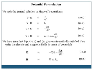
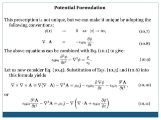
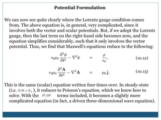
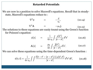
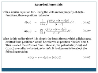
POTENTIAL AND FIELDS
By:
DR. SAKTIOTO, M.PHIL
Potential Formulation
We seek the general solution to Maxwell’s equations:
We have seen that Eqs. (10.2) and (10.3) are automatically satisfied if we
write the electric and magnetic fields in terms of potentials
(10.1)
(10.2)
(10.3)
(10.4)
(10.5)
(10.6)
Potential Formulation
This prescription is not unique, but we can make it unique by adopting the
following conventions:
The above equations can be combined with Eq. (10.1) to give:
Let us now consider Eq. (10.4). Substitution of Eqs. (10.5) and (10.6) into
this formula yields
or
(10.7)
(10.8)
(10.9)
(10.10)
(10.11)
Potential Formulation
We can now see quite clearly where the Lorentz gauge condition comes
from. The above equation is, in general, very complicated, since it
involves both the vector and scalar potentials. But, if we adopt the Lorentz
gauge, then the last term on the right-hand side becomes zero, and the
equation simplifies considerably, such that it only involves the vector
potential. Thus, we find that Maxwell's equations reduce to the following:
This is the same (scalar) equation written four times over. In steady-state
(i.e. , ), it reduces to Poisson's equation, which we know how to
solve. With the terms included, it becomes a slightly more
complicated equation (in fact, a driven three-dimensional wave equation).
(10.12)
(10.13)
Retarded Potentials
We are now in a position to solve Maxwell's equations. Recall that in steady-
state, Maxwell's equations reduce to :
The solutions to these equations are easily found using the Green's function
for Poisson's equation:
We can solve these equations using the time-dependent Green's function :
(10.14)
(10.15)
(10.16)
(10.17)
(10.18)
Retarded Potentials
with a similar equation for . Using the well-known property of delta-
functions, these equations reduce to
What is this earlier time? It is simply the latest time at which a light signal
emitted from position r’ would be received at position r before time t .
This is called the retarded time. Likewise, the potentials (10.19) and
(10.20) are called retarded potentials. It is often useful to adopt the
following notation
(10.19)
(10.20)
(10.21)

potential and fields

  • 1.
  • 2.
    Potential Formulation We seekthe general solution to Maxwell’s equations: We have seen that Eqs. (10.2) and (10.3) are automatically satisfied if we write the electric and magnetic fields in terms of potentials (10.1) (10.2) (10.3) (10.4) (10.5) (10.6)
  • 3.
    Potential Formulation This prescriptionis not unique, but we can make it unique by adopting the following conventions: The above equations can be combined with Eq. (10.1) to give: Let us now consider Eq. (10.4). Substitution of Eqs. (10.5) and (10.6) into this formula yields or (10.7) (10.8) (10.9) (10.10) (10.11)
  • 4.
    Potential Formulation We cannow see quite clearly where the Lorentz gauge condition comes from. The above equation is, in general, very complicated, since it involves both the vector and scalar potentials. But, if we adopt the Lorentz gauge, then the last term on the right-hand side becomes zero, and the equation simplifies considerably, such that it only involves the vector potential. Thus, we find that Maxwell's equations reduce to the following: This is the same (scalar) equation written four times over. In steady-state (i.e. , ), it reduces to Poisson's equation, which we know how to solve. With the terms included, it becomes a slightly more complicated equation (in fact, a driven three-dimensional wave equation). (10.12) (10.13)
  • 5.
    Retarded Potentials We arenow in a position to solve Maxwell's equations. Recall that in steady- state, Maxwell's equations reduce to : The solutions to these equations are easily found using the Green's function for Poisson's equation: We can solve these equations using the time-dependent Green's function : (10.14) (10.15) (10.16) (10.17) (10.18)
  • 6.
    Retarded Potentials with asimilar equation for . Using the well-known property of delta- functions, these equations reduce to What is this earlier time? It is simply the latest time at which a light signal emitted from position r’ would be received at position r before time t . This is called the retarded time. Likewise, the potentials (10.19) and (10.20) are called retarded potentials. It is often useful to adopt the following notation (10.19) (10.20) (10.21)