Downloaded 13 times
![5
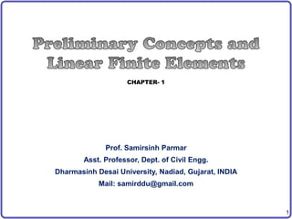
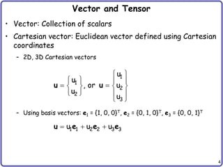
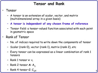
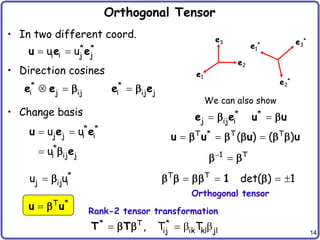
Index Notation and Summation Rule
• Index notation: Any vector or matrix can be expressed in
terms of its indices
• Einstein summation convention
– In this case, k is a dummy variable (can be j or i)
– The same index cannot appear more than twice
• Basis representation of a vector
– Let ek be the basis of vector space V
– Then, any vector in V can be represented by
3
k k k k
k 1
a b a b
N
k k k k
k 1
w w
w e e
1 11 12 13
i 2 ij 21 22 23
3 31 32 33
v A A A
[v ] v [A ] A A A
v A A A
v A](https://image.slidesharecdn.com/chap-1preliminaryconceptsandlinearfiniteelements-230201055401-ceccf7ce/85/Chap-1-Preliminary-Concepts-and-Linear-Finite-Elements-pptx-5-320.jpg)
![10
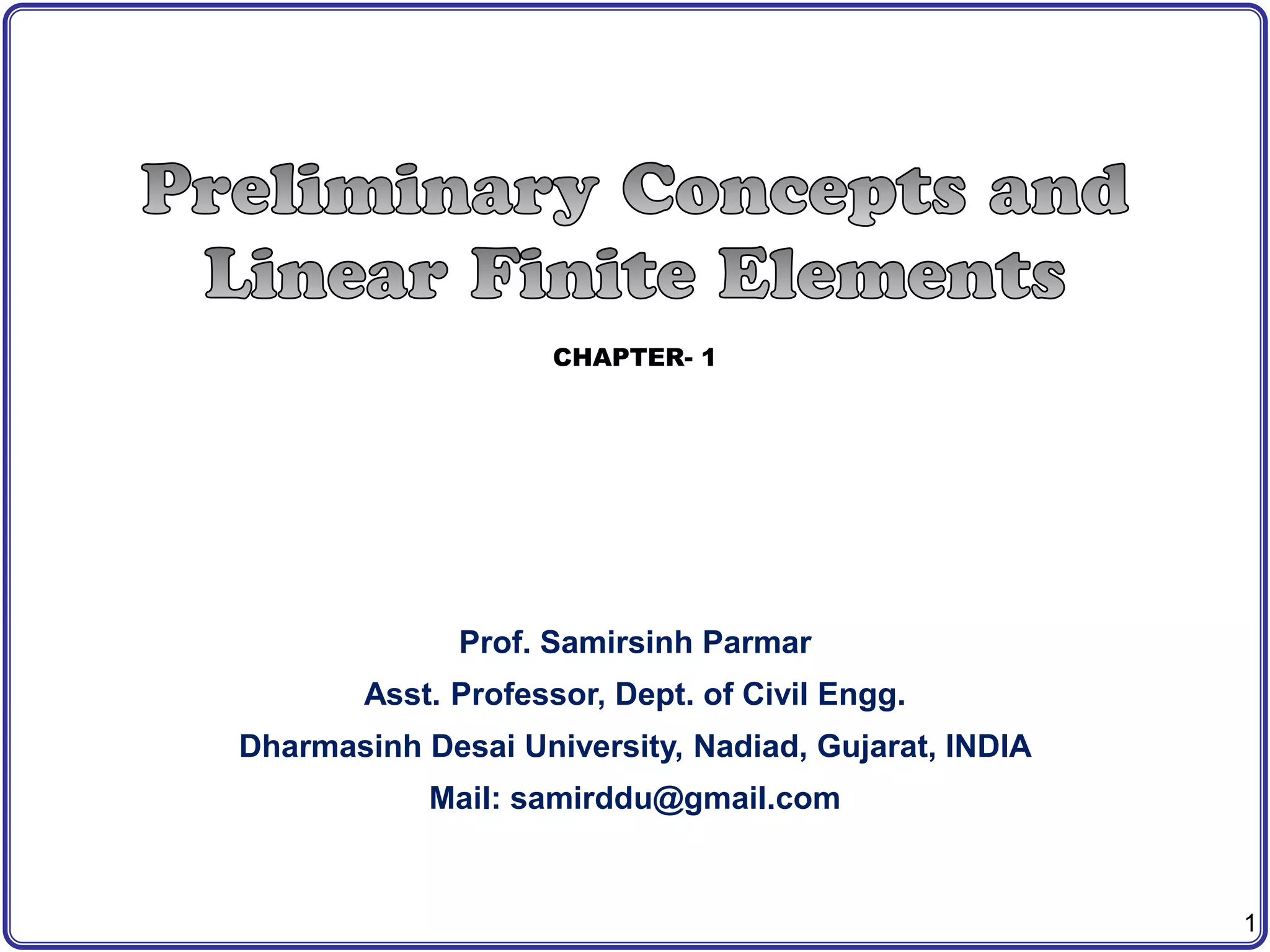
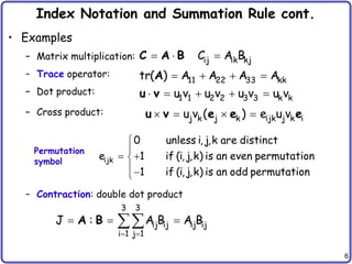
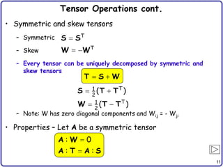
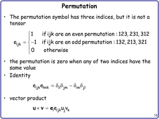
Tensor Operations
• Basic rules for tensors
• Tensor (dyadic) product: increase rank
i j i j ij i j
uv A uv
A u v e e
( ) ( )
( ) ( )
( )( ) ( )
u v w u v w
w u v v w u
u v w x v w u x
u v v u
( ) ( )
( )
( ) ( ) ( )
TS R T SR
T S R TS TR
TS T S T S
1T T1 T
Different notations
TS T S
Identity tensor
ij
[ ]
1](https://image.slidesharecdn.com/chap-1preliminaryconceptsandlinearfiniteelements-230201055401-ceccf7ce/85/Chap-1-Preliminary-Concepts-and-Linear-Finite-Elements-pptx-10-320.jpg)
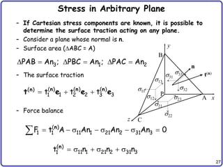
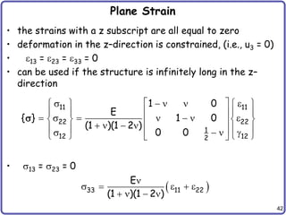
![26
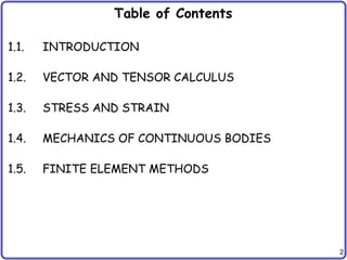
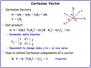
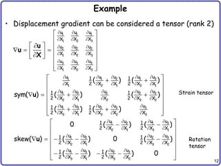
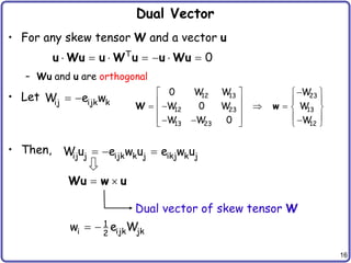
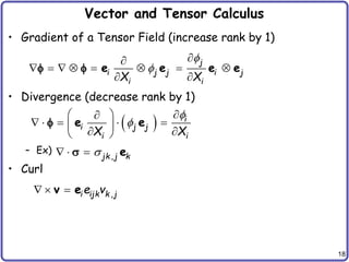
Symmetry of Stress Tensor
– Stress tensor should be symmetric
9 components 6 components
– Equilibrium of the angular moment
– Similarly for all three directions:
– Let’s use vector notation:
12
21
x
y
12
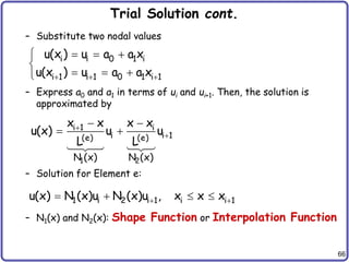
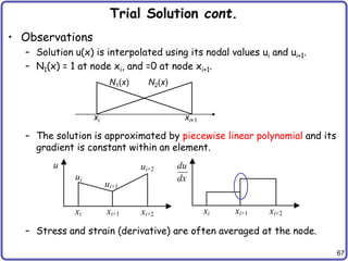
21
O
l
l
A B
C D
12 21
12 21
M l( ) 0
11 12 13
ij 12 22 23
13 23 33
[ ]
11
22
33
12
23
13
{ }
12 21 23 32 13 31
, ,
Cartesian components
of stress tensor](https://image.slidesharecdn.com/chap-1preliminaryconceptsandlinearfiniteelements-230201055401-ceccf7ce/85/Chap-1-Preliminary-Concepts-and-Linear-Finite-Elements-pptx-26-320.jpg)
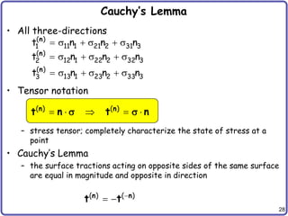
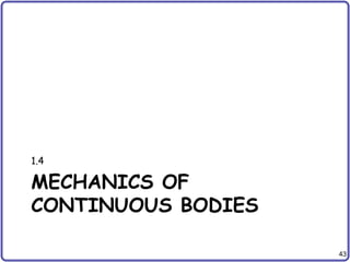
![33
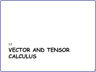
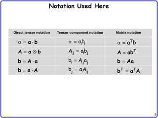
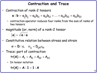
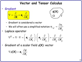
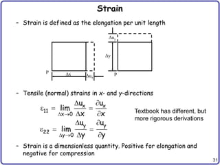
Strain Tensor
• Strain Tensor
• Cartesian Components
• Vector notation
ij i j
e e
11 12 13
ij 12 22 23
13 23 33
[ ]
11 11
22 22
33 33
12 12
23 23
13 13
{ }
2
2
2
g
g
g
](https://image.slidesharecdn.com/chap-1preliminaryconceptsandlinearfiniteelements-230201055401-ceccf7ce/85/Chap-1-Preliminary-Concepts-and-Linear-Finite-Elements-pptx-33-320.jpg)
![37
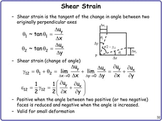
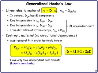
Generalized Hooke’s Law cont.
• Stress-strain relation
– Volumetric strain:
– Off-diagonal part:
– Bulk modulus K: relation b/w volumetric stress & strain
– Substitute so that we can separate volumetric part
• Total deform. = volumetric + deviatoric deform.
ij ijkl kl ij kl ik jl il jk kl kk ij ij
D [ ( )] 2
kk 11 22 33 v
12 12 12
2
g is the shear modulus
1 m jj kk jj jj kk
I 3 2 (3 2 )
2
m kk v
3
( ) K
Bulk modulus
2
3
K
](https://image.slidesharecdn.com/chap-1preliminaryconceptsandlinearfiniteelements-230201055401-ceccf7ce/85/Chap-1-Preliminary-Concepts-and-Linear-Finite-Elements-pptx-37-320.jpg)
![38
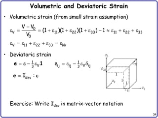
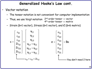
Generalized Hooke’s Law cont.
• Stress-strain relation cont.
2
ij kk ij ij
3
2
kk ij ij kk ij
3
1
ij kl kl ik jl ij kl kl
3
ij kl dev ijkl kl
(K ) 2
K 2
K 2 [ ]
K 2 (I )
dev
σ K 2 : ε
1 1 I
Deviatoric part
Volumetric part
v
m
σ K 2
σ
1 e
1 s
dev :
e I
Deviatoric strain
Important for plasticity; plastic deformation only occurs in deviatoric part
volumetric part is always elastic
dev :
s I
Deviatoric stress](https://image.slidesharecdn.com/chap-1preliminaryconceptsandlinearfiniteelements-230201055401-ceccf7ce/85/Chap-1-Preliminary-Concepts-and-Linear-Finite-Elements-pptx-38-320.jpg)
![45
Balance of Linear Momentum cont
• Balance of linear momentum
– For a static problem
• Balance of angular momentum
b
( )d d d
f a n
b
[ ( )]d 0
f a
b
( ) 0
f a
b b
ij,i j
0 f 0
f
b
d d d
n
x f x t x a
T
ij ji
Divergence Thm](https://image.slidesharecdn.com/chap-1preliminaryconceptsandlinearfiniteelements-230201055401-ceccf7ce/85/Chap-1-Preliminary-Concepts-and-Linear-Finite-Elements-pptx-45-320.jpg)
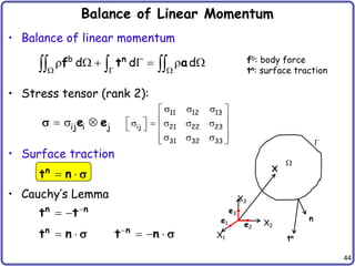
![46
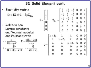
Boundary-Valued Problem
• We want to determine the state of a body in equilibrium
• The equilibrium state (solution) of the body must satisfy
– local momentum balance equation
– boundary conditions
• Strong form of BVP
– Given body force fb, and traction t
on the boundary, find u such that
and
• Solution space
h
s
on essential BC
on natural BC
u 0
t n
b
0
f
(1)
(2)
(3)
n
t
X1
X2
X3
e1 e2
e3
X
fb
2 3 h s
A
D [C ( )] | 0 on , on
u u x n t x
](https://image.slidesharecdn.com/chap-1preliminaryconceptsandlinearfiniteelements-230201055401-ceccf7ce/85/Chap-1-Preliminary-Concepts-and-Linear-Finite-Elements-pptx-46-320.jpg)
![50
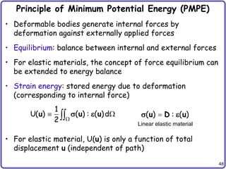
PMPE cont.
• PMPE: for all displacements that satisfy the boundary
conditions, known as kinematically admissible
displacements, those which satisfy the boundary-valued
problem make the total potential energy stationary on DA
• But, the potential energy is well defined in the space of
kinematically admissible displacements
• No need to satisfy traction BC (it is a part of potential)
• Less requirement on continuity
• The solution is called a generalized (natural) solution
1 3 h
[H ( )] | 0 on ,
u u x
Z
H1: first-order derivatives are integrable](https://image.slidesharecdn.com/chap-1preliminaryconceptsandlinearfiniteelements-230201055401-ceccf7ce/85/Chap-1-Preliminary-Concepts-and-Linear-Finite-Elements-pptx-50-320.jpg)
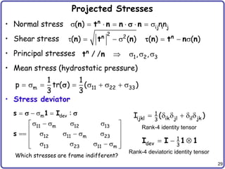
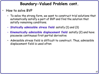
![51
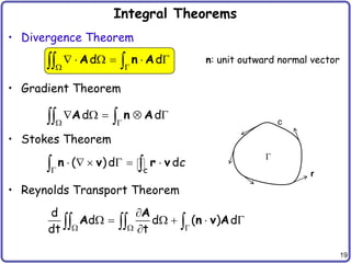
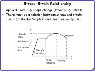
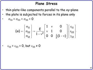
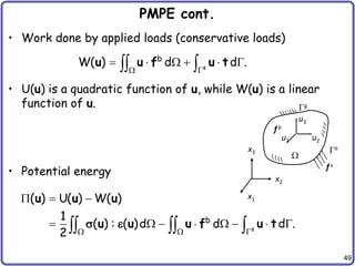
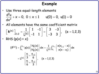
Example – Uniaxial Bar
• Strong form
• Integrate twice:
• Apply two BCs:
• PMPE with assumed solution u(x) = c1x + c2
• To satisfy KAD space, u(0) = 0, u(x) = c1x
• Potential energy:
L
F
x
EAu 0 x [0,L]
u 0 x 0
EAu (L) F x L
1 2
EAu(x) c x c
Fx
u(x)
EA
L 2 2
1
0
1
1
U EA(u ) dx EALc
2
W Fu(L) FLc
1
1 1
d d
(U W) EALc FL 0
dc dc
1
F Fx
c u(x)
EA EA
](https://image.slidesharecdn.com/chap-1preliminaryconceptsandlinearfiniteelements-230201055401-ceccf7ce/85/Chap-1-Preliminary-Concepts-and-Linear-Finite-Elements-pptx-51-320.jpg)
![52
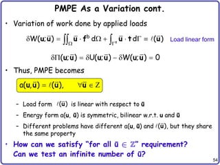
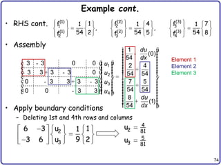
Virtual Displacement Field
• Virtual displacement (Space Z)
– Small arbitrary perturbation (variation) of real displacement
– Let ū be the virtual displacement, then u + ū must be kinematically
admissible, too
– Then, ū must satisfy homogeneous displacement BC
– Space Z only includes homogeneous
essential BCs
• Property of variation
u u u u
V Z
h
1 3
[H ( )] , 0
u u u
Z
In the literature, u is often used instead of ū
d d( )
dx dx
u u
0
0
1 d
lim [( ) ( )] ( ) .
d
u u u u u
](https://image.slidesharecdn.com/chap-1preliminaryconceptsandlinearfiniteelements-230201055401-ceccf7ce/85/Chap-1-Preliminary-Concepts-and-Linear-Finite-Elements-pptx-52-320.jpg)
![53
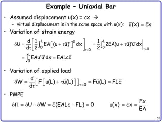
PMPE As a Variation
• Necessary condition for minimum PE
– Stationary condition <--> first variation = 0
• Variation of strain energy
0
0
1 d
( ; ) lim [ ( ) ( )] ( ) 0
d
u u u u u u u
Z
for all u
0
d
d
u u u u
x x x
( ) ( )
u u
:
D
1
2
U( ; ) ( ) : : ( ) ( ) : : ( ) d
( ) : : ( )d
a( , )
u u u D u u D u
u D u
u u
Energy bilinear form](https://image.slidesharecdn.com/chap-1preliminaryconceptsandlinearfiniteelements-230201055401-ceccf7ce/85/Chap-1-Preliminary-Concepts-and-Linear-Finite-Elements-pptx-53-320.jpg)
![58
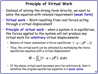
Principle of Virtual Work cont
• Since ij is symmetric
• Weak Form of BVP
Internal virtual work = external virtual work
Starting point of FEM
• Symbolic expression
– Energy form:
– Load form:
s
b
ij ij j j j j
d f u d t u d
u Z
a( , ) ( )
u u u u Z
a( , ) : d
u u
s
b
( ) d d
u u f u t
ij j,i ij j,i ij ij
u sym(u )
j
i
i,j ij
j i
u
u
1
sym(u )
2 X X
[ ]{ } { }
K d F
FE equation](https://image.slidesharecdn.com/chap-1preliminaryconceptsandlinearfiniteelements-230201055401-ceccf7ce/85/Chap-1-Preliminary-Concepts-and-Linear-Finite-Elements-pptx-58-320.jpg)
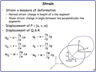
![60
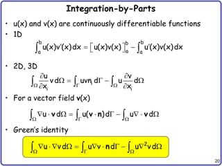
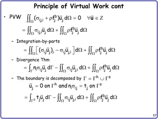
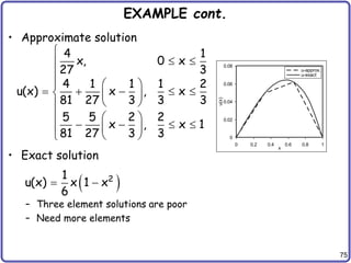
Example – Beam Problem
• Governing DE
• Boundary conditions for cantilevered beam
• Space of kinematically admissible displacement
• Integrate-by-part twice, and apply BCs
4
4
d v
EI f(x), x [0,L]
dx
2 3
2 3
dv d v d v
v(0) (0) (L) (L) 0
dx dx dx
f(x)
x L
2 dv
v H [0,L] v(0) (0) 0
dx
Z
2 2
L L
2 2
0 0
d v d v
EI dx fv dx, v
dx dx
Z](https://image.slidesharecdn.com/chap-1preliminaryconceptsandlinearfiniteelements-230201055401-ceccf7ce/85/Chap-1-Preliminary-Concepts-and-Linear-Finite-Elements-pptx-60-320.jpg)
![68
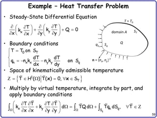
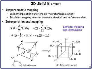
1D Finite Elements
• 1D BVP
• Use PVW
• Integration-by-parts
– This variational equation also satisfies at individual element level
2
2
d u
p(x) 0, 0 x 1s
dx
u(0) 0
Boundary conditions
du
(1) 0
dx
2
1
2
0
d u
p u dx 0
dx
(1)
u H [0,1] u(0) 0
Z
Space of kinematically
admissible displacements
1
1 1
0 0
0
du du du
u dx pu dx
dx dx dx
](https://image.slidesharecdn.com/chap-1preliminaryconceptsandlinearfiniteelements-230201055401-ceccf7ce/85/Chap-1-Preliminary-Concepts-and-Linear-Finite-Elements-pptx-68-320.jpg)
![70
Element-Level Variational Equation
• Approximate variational equation for element (e)
– Must satisfied for all
– If element (e) is not on the boundary, can be arbitrary
• Element-level variational equation
j j
i i
i
x x
(e)T (e)T (e) (e) (e)T (e)T (e)T
x x
i 1
du
(x )
dx
dx p(x)dx
du
(x )
dx
d B B d d N d
(e)
u (x) Z
(e)
d
j j
i i
i
x x
(e)T (e) (e) (e)T
x x
i 1
du
(x )
dx
dx p(x)dx
du
(x )
dx
B B d N
i
(e) (e) (e)
i 1
du
(x )
dx
[ ]{ }
du
(x )
dx
k d f
2x2 matrix 2x1 vector](https://image.slidesharecdn.com/chap-1preliminaryconceptsandlinearfiniteelements-230201055401-ceccf7ce/85/Chap-1-Preliminary-Concepts-and-Linear-Finite-Elements-pptx-70-320.jpg)
![72
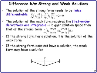
Assembly cont.
• Assembly of NE elements (ND = NE + 1)
• Coefficient matrix [K] is singular; it will become non-
singular after applying boundary conditions
E E
E
D
D
D D
(1) (1) (1)
11 12 1
1
(1) (1) (2) (2) (1) (2)
21 22 11 12 2 2
2
(2) (2) (2) (2) (3)
3
221 22 11 3 3
N (N )
(N )
N N
21 22 N 1 N 1
N N
k k 0 0 f
u
k k k k 0 f f
u
u
0 k k k 0 f f
u f
0 0 0 k k
D
1
N
N 1
du
(x )
dx
0
0
du
(x )
dx
[ ]{ } { }
K q F](https://image.slidesharecdn.com/chap-1preliminaryconceptsandlinearfiniteelements-230201055401-ceccf7ce/85/Chap-1-Preliminary-Concepts-and-Linear-Finite-Elements-pptx-72-320.jpg)
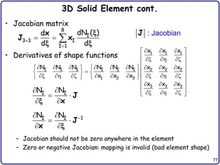
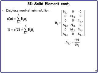
![79
3D Solid Element cont.
• Transformation of integration domain
• Energy form
• Load form
• Discrete variational equation
1 1 1
1 1 1
d d d d
x z
J
8 8
1 1 1
T T T
I I J J
1 1 1
I 1 J 1
a( , ) d d d { } [ ]{ }
x z
u u u B DB J u d k d
8
1 1 1
T b T
I I
1 1 1
I 1
( ) N ( ) d d d { } { }
x z
u u f J d f
x
T T
h
{ } [ ]{ } { } { }, { }
d k d d f d Z](https://image.slidesharecdn.com/chap-1preliminaryconceptsandlinearfiniteelements-230201055401-ceccf7ce/85/Chap-1-Preliminary-Concepts-and-Linear-Finite-Elements-pptx-79-320.jpg)
![80
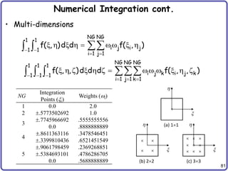
Numerical Integration
• For bar and beam, analytical integration is possible
• For plate and solid, analytical integration is difficult, if
not impossible
• Gauss quadrature is most popular in FEM due to simplicity
and accuracy
• 1D Gauss quadrature
– NG: No. of integ. points; xi: integ. point; wi: integ. weight
– xi and wi are chosen so that the integration is exact
for (2NG – 1)-order polynomial
– Works well for smooth function
– Integration domain is [-1, 1]
NG
1
i i
1
i 1
f( )d f( )
x x w x
](https://image.slidesharecdn.com/chap-1preliminaryconceptsandlinearfiniteelements-230201055401-ceccf7ce/85/Chap-1-Preliminary-Concepts-and-Linear-Finite-Elements-pptx-80-320.jpg)


The document is a detailed overview of vector and tensor calculus, including topics such as definitions of vectors, index notation, tensor operations, and the mechanics of continuous bodies. It covers fundamental concepts including stress and strain, finite element methods, and integral theorems relevant to engineering applications. The content serves as an educational resource for students in the field of civil engineering, specifically focusing on mathematical methods necessary for understanding structural mechanics.


![[Deck] What's New in Spark-Iceberg Integration via DSV2.pptx](https://cdn.slidesharecdn.com/ss_thumbnails/deckwhatsnewinspark-icebergintegrationviadsv2-260210005337-25955b12-thumbnail.jpg?width=640&height=640&fit=bounds)


