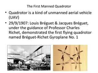
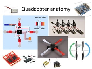
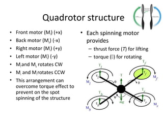
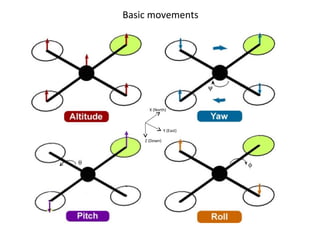
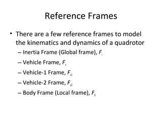
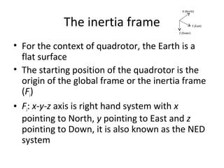
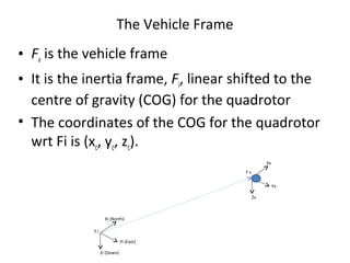
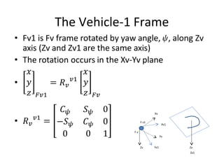
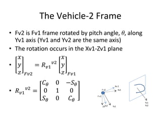
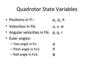
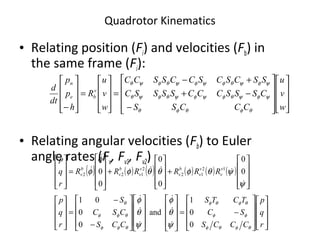
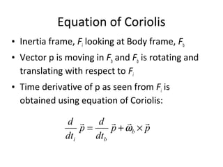
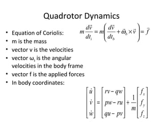
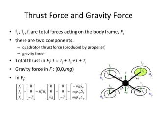
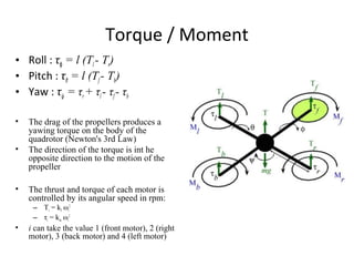
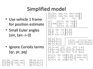
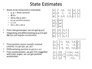
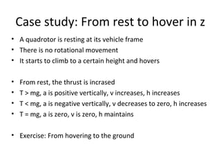
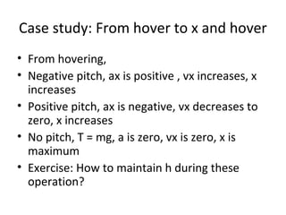
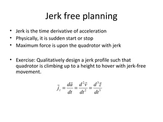
Chapter 3
Quadrotor / Quadcopter
The First Manned Quadrotor
• Quadrotor is a kind of unmanned aerial vehicle
(UAV)
• 29/9/1907: Louis Bréguet & Jacques Bréguet,
under the guidance of Professor Charles
Richet, demonstrated the first flying quadrotor
named Bréguet-Richet Gyroplane No. 1
Advantages of quadrotor
• Quadrotor is a rotary wing UAV
• Its advantages over fixed wing UAVs:
– Vertical Take Off and Landing (VTOL)
– Able to hover
– Able to make slow precise movements.
– Four rotors provide a higher payload capacity
– More flexible in maneuverability through an
environment with many obstacles, or landing in
small areas.
Quadcopter anatomy
Quadrotor structure
• Front motor (Mf) (+x)
• Back motor (Mb) (-x)
• Right motor (Mr) (+y)
• Left motor (Ml) (-y)
• Mfand Mb rotates CW
• Mr and Mlrotates CCW
• This arrangement can
overcome torque effect to
prevent on the spot
spinning of the structure
• Each spinning motor
provides
– thrust force (T) for lifting
– torque () for rotating
Basic movements
X (North)
Y (East)
Z (Down)
Reference Frames
• There are a few reference frames to model
the kinematics and dynamics of a quadrotor
– Inertia Frame (Global frame), Fi
– Vehicle Frame, Fv
– Vehicle-1 Frame, Fv1
– Vehicle-2 Frame, Fv2
– Body Frame (Local frame), Fb
The inertia frame
• For the context of quadrotor, the Earth is a
flat surface
• The starting position of the quadrotor is the
origin of the global frame or the inertia frame
(Fi)
• Fi: x-y-z axis is right hand system with x
pointing to North, y pointing to East and z
pointing to Down, it is also known as the NED
system
X (North)
Y (East)
Z (Down)
The Vehicle Frame
• Fv is the vehicle frame
• It is the inertia frame, Fi, linear shifted to the
centre of gravity (COG) for the quadrotor
• The coordinates of the COG for the quadrotor
wrt Fi is (xc, yc, zc).
Xi (North)
Yi (East)
Zi (Down)
Xv
Yv
Zv
F v
F i
The Vehicle-1 Frame
Xv
Yv
Zv
F v
F v1
Zv
Zv1
Yv1
Xv1
The Vehicle-2 Frame
Xv 2
Zv2Zv
F v1
F v2
Yv1
Yv2Yv1
Xv1
The Body Frame
Xv 2
Zv2
Zb
F v2
F b
Xv2
Xb
Yv2Yb
Vehicle Frame  Body Frame
, ,  are known as Euler angles. They are measured from different frames (Roll in
Fv2 frame, Pitch in Fv1 frame, Yaw in Fv frame)
Gimbal Lock
• This is a fundamental problem when
using sensors to sense Euler angles
• When pitch angle is 90 degrees, roll and
yaw rotation give the same sensor
readings
• Information for 1 dimension is lost and
the actual configuration of the rigid body
is not correctly sensed
• Solution:
– Avoid 90 degree pitch when using Euler
angle sensor
Quadrotor State Variables
• Positions in Fi : pn, pe, h
• Velocities in Fb: u, v, w
• Angular velocities in Fb: p, q, r
• Euler angles:
– Yaw angle in Fv: ψ
– Pitch angle in Fv1: θ
– Roll angle in Fv2: ϕ
Quadrotor Kinematics




















−
−+
+−
=










=










− w
v
u
CCCSS
CSSSCCCSSSSC
SSCSCSCCSSCC
w
v
u
R
h
p
p
dt
d v
be
n
θφθφθ
ψφψθφψφψθφψθ
ψφψθφψφψθφψθ
( ) ( ) ( ) ( ) ( ) ( )




















−=






























−
−
=




















+










+










=










r
q
p
CCCS
SC
TCTS
CCS
CSC
S
r
q
p
RRRRRR
r
q
p
v
v
v
v
b
v
v
v
b
v
b
v
θφθφ
φφ
θφθφ
θφφ
θφφ
θ
ψ
θ
φ
ψ
θ
φ
ψ
ψθφθθφ
φ
φ
0
0
1
and
0
0
01
0
0
0
0
0
0 12
12
2
122










• Relating position (Fi) and velocities (Fb) in
the same frame (Fi):
• Relating angular velocities (Fb) to Euler
angle rates (Fv, Fv1, Fv2)
Equation of Coriolis
pp
dt
d
p
dt
d
b
bi

×+= ω
• Inertia frame, Fi looking at Body frame, Fb
• Vector p is moving in Fb and Fb is rotating and
translating with respect to Fi
• Time derivative of p as seen from Fi is
obtained using equation of Coriolis:
Quadrotor Dynamics
• Equation of Coriolis:
• m is the mass
• vector v is the velocities
• vector ωb is the angular
velocities in the body frame
• vector f is the applied forces
• In body coordinates:










+










−
−
−
=










z
y
x
f
f
f
m
pvqu
rupw
qwrv
w
v
u
1



fv
dt
vd
m
dt
vd
m b
bi


=





×+= ω
Rotational Motion
• Equation of Coriolis for rotational motion:
• vector h is angular momentum, h = Jωb
• J is symmetric inertia matrix
• vector m is the applied torque
• Substitutes into equation of Coriolis:
• Angular acceleration is hence given by:
mhh
dt
d
h
dt
d
b
bi

=×+= ω










=










=










=
ψ
θ
φ
τ
τ
τ
ω m
r
q
p
I
I
I
J b
z
y
x

;;
00
00
00
{ }
{ }
{ } 









+−
+−
+−
=




















=










×










+










zyx
yxz
xzy
IpqII
IprII
IqrII
r
q
p
r
q
p
J
r
q
p
r
q
p
J
ψ
θ
φ
ψ
θ
φ
τ
τ
τ
τ
τ
τ
)(
)(
)(






Summary of Equation Set




















−
−+
+−
=










− w
v
u
CCCSS
CSSSCCCSSSSC
SSCSCSCCSSCC
h
p
p
e
n
θφθφθ
ψφψθφψφψθφψθ
ψφψθφψφψθφψθ























−=










r
q
p
CCCS
SC
TCTS
θφθφ
φφ
θφθφ
ψ
θ
φ
0
0
1



{ }
{ }
{ } 









+−
+−
+−
=










zyx
yxz
xzy
IpqII
IprII
IqrII
r
q
p
ψ
θ
φ
τ
τ
τ
)(
)(
)(













+










−
−
−
=










z
y
x
f
f
f
m
pvqu
rupw
qwrv
w
v
u
1



Thrust Force and Gravity Force
• fx , fy , fz are total forces acting on the body frame, Fb
• there are two components:
– quadrotor thrust force (produced by propeller)
– gravity force
• Total thrust in Fb: T = Tf + Tb +Tl + Tr
• Gravity force in Fi : (0,0,mg)
• In Fb:









 −
+










−
=










+










−
=










φθ
φθ
θ
CmgC
SmgC
mgS
Tmg
RR
Tf
f
f
v
i
b
v
z
y
x
0
0
0
0
0
0
Torque / Moment
• Roll : τϕ = l (Tl - Tr)
• Pitch : τθ = l (Tf- Tb)
• Yaw : τψ = τr+ τl- τf- τb
• The drag of the propellers produces a
yawing torque on the body of the
quadrotor (Newton's 3rd Law)
• The direction of the torque is int he
opposite direction to the motion of the
propeller
• The thrust and torque of each motor is
controlled by its angular speed in rpm:
– Ti = kf ωi
2
– τi = km ωi
2
• i can take the value 1 (front motor), 2 (right
motor), 3 (back motor) and 4 (left motor)
Simplified model
• Use vehicle 1 frame
for position estimate
• Small Euler angles
(sin, tan -> 0)
• Ignore Coriolis terms
(qr, pr, pq)




















−−
−+
+−
=










w
v
u
CCCSS
CSSSCCCSSSSC
SSCSCSCCSSCC
h
p
p
e
n
θφθφθ
ψφψθφψφψθφψθ
ψφψθφψφψθφψθ












 −
+










−
=










=










+










−
−
−
=










φθ
φθ
θ
CC
SC
S
g
T
m
f
f
f
m
f
f
f
m
pvqu
rupw
qwrv
w
v
u
z
y
x
z
y
x
0
0
111













=




















−=










r
q
p
r
q
p
CCCS
SC
TCTS
θφθφ
φφ
θφθφ
ψ
θ
φ
0
0
1













=










=










z
y
x
I
I
I
r
q
p
ψ
θ
φ
τ
τ
τ
ψ
θ
φ


























−
−=










=










w
v
u
CCCSS
SC
SCSSC
w
v
u
RR
p
p
p
v
b
v
v
z
y
x
θφθφθ
φφ
θφθφθ
021
2













−
+−
−−
+










=




















−
−=










θφ
ψφψθφ
ψφψθφ
θφθφθ
φφ
θφθφθ
CC
CSSSC
SSCSC
m
T
gw
v
u
CCCSS
SC
SCSSC
p
p
p
z
y
x
0
0
0















 −
+










−
=










+










−
=










φθ
φθ
θ
CmgC
SmgC
mgS
Tmg
RR
Tf
f
f
v
i
b
v
z
y
x
0
0
0
0
0
0










=










=










z
y
x
I
I
I
r
q
p
ψ
θ
φ
τ
τ
τ
ψ
θ
φ
















−
+−
−−
+










=










θφ
ψφψθφ
ψφψθφ
CC
CSSSC
SSCSC
m
T
gp
p
p
z
y
x
0
0



State Estimates
• States to be measured or estimated:
– p, q, r (from sensors)
– ,θ,ψϕ
– dot p, dot q, dot r
– px, py, pz (from sensors)
– u, v, w
– dot u, dot v, dot w
• From rate gyroscopes, we can get (p,q,r)
• Integrating and differentiating (p,q,r) to get
( ,θ,ψ) and angular accelerationϕ
• From position sensor (usually external
camera), we get (px, py, pz)
• Differentiating position to get (u,v,w)
• From accelerometer, we get T/m, toggether
with Euler angles, we can get position
acceleration










=










=










z
y
x
I
I
I
r
q
p
ψ
θ
φ
τ
τ
τ
ψ
θ
φ
















−
+−
−−
+










=










θφ
ψφψθφ
ψφψθφ
CC
CSSSC
SSCSC
m
T
gp
p
p
z
y
x
0
0













=




















−=










r
q
p
r
q
p
CCCS
SC
TCTS
θφθφ
φφ
θφθφ
ψ
θ
φ
0
0
1























−
−=










w
v
u
CCCSS
SC
SCSSC
p
p
p
z
y
x
θφθφθ
φφ
θφθφθ
0















=










∫
∫
∫
rdt
qdt
pdt
ψ
θ
φ
Case study: From rest to hover in z
• A quadrotor is resting at its vehicle frame
• There is no rotational movement
• It starts to climb to a certain height and hovers
• From rest, the thrust is incrased
• T > mg, a is positive vertically, v increases, h increases
• T < mg, a is negative vertically, v decreases to zero, h increases
• T = mg, a is zero, v is zero, h maintains
• Exercise: From hovering to the ground
Case study: From hover to x and hover
• From hovering,
• Negative pitch, ax is positive , vx increases, x
increases
• Positive pitch, ax is negative, vx decreases to
zero, x increases
• No pitch, T = mg, a is zero, vx is zero, x is
maximum
• Exercise: How to maintain h during these
operation?
Jerk free planning
• Jerk is the time derivative of acceleration
• Physically, it is sudden start or stop
• Maximum force is upon the quadrotor with jerk
• Exercise: Qualitatively design a jerk profile such that
quadrotor is climbing up to a height to hover with jerk-free
movement.
3
3
2
2
dt
zd
dt
vd
dt
ad
jz

===

Lecture 1: Quadrotor

  • 1.
  • 2.
    The First MannedQuadrotor • Quadrotor is a kind of unmanned aerial vehicle (UAV) • 29/9/1907: Louis Bréguet & Jacques Bréguet, under the guidance of Professor Charles Richet, demonstrated the first flying quadrotor named Bréguet-Richet Gyroplane No. 1
  • 3.
    Advantages of quadrotor •Quadrotor is a rotary wing UAV • Its advantages over fixed wing UAVs: – Vertical Take Off and Landing (VTOL) – Able to hover – Able to make slow precise movements. – Four rotors provide a higher payload capacity – More flexible in maneuverability through an environment with many obstacles, or landing in small areas.
  • 4.
  • 5.
    Quadrotor structure • Frontmotor (Mf) (+x) • Back motor (Mb) (-x) • Right motor (Mr) (+y) • Left motor (Ml) (-y) • Mfand Mb rotates CW • Mr and Mlrotates CCW • This arrangement can overcome torque effect to prevent on the spot spinning of the structure • Each spinning motor provides – thrust force (T) for lifting – torque () for rotating
  • 6.
  • 7.
    Reference Frames • Thereare a few reference frames to model the kinematics and dynamics of a quadrotor – Inertia Frame (Global frame), Fi – Vehicle Frame, Fv – Vehicle-1 Frame, Fv1 – Vehicle-2 Frame, Fv2 – Body Frame (Local frame), Fb
  • 8.
    The inertia frame •For the context of quadrotor, the Earth is a flat surface • The starting position of the quadrotor is the origin of the global frame or the inertia frame (Fi) • Fi: x-y-z axis is right hand system with x pointing to North, y pointing to East and z pointing to Down, it is also known as the NED system X (North) Y (East) Z (Down)
  • 9.
    The Vehicle Frame •Fv is the vehicle frame • It is the inertia frame, Fi, linear shifted to the centre of gravity (COG) for the quadrotor • The coordinates of the COG for the quadrotor wrt Fi is (xc, yc, zc). Xi (North) Yi (East) Zi (Down) Xv Yv Zv F v F i
  • 10.
    The Vehicle-1 Frame Xv Yv Zv Fv F v1 Zv Zv1 Yv1 Xv1
  • 11.
    The Vehicle-2 Frame Xv2 Zv2Zv F v1 F v2 Yv1 Yv2Yv1 Xv1
  • 12.
    The Body Frame Xv2 Zv2 Zb F v2 F b Xv2 Xb Yv2Yb
  • 13.
  • 14.
    , , are known as Euler angles. They are measured from different frames (Roll in Fv2 frame, Pitch in Fv1 frame, Yaw in Fv frame)
  • 15.
    Gimbal Lock • Thisis a fundamental problem when using sensors to sense Euler angles • When pitch angle is 90 degrees, roll and yaw rotation give the same sensor readings • Information for 1 dimension is lost and the actual configuration of the rigid body is not correctly sensed • Solution: – Avoid 90 degree pitch when using Euler angle sensor
  • 16.
    Quadrotor State Variables •Positions in Fi : pn, pe, h • Velocities in Fb: u, v, w • Angular velocities in Fb: p, q, r • Euler angles: – Yaw angle in Fv: ψ – Pitch angle in Fv1: θ – Roll angle in Fv2: ϕ
  • 17.
    Quadrotor Kinematics                     − −+ +− =           =           − w v u CCCSS CSSSCCCSSSSC SSCSCSCCSSCC w v u R h p p dt dv be n θφθφθ ψφψθφψφψθφψθ ψφψθφψφψθφψθ ( ) ( ) ( ) ( ) ( ) ( )                     −=                               − − =                     +           +           =           r q p CCCS SC TCTS CCS CSC S r q p RRRRRR r q p v v v v b v v v b v b v θφθφ φφ θφθφ θφφ θφφ θ ψ θ φ ψ θ φ ψ ψθφθθφ φ φ 0 0 1 and 0 0 01 0 0 0 0 0 0 12 12 2 122           • Relating position (Fi) and velocities (Fb) in the same frame (Fi): • Relating angular velocities (Fb) to Euler angle rates (Fv, Fv1, Fv2)
  • 18.
    Equation of Coriolis pp dt d p dt d b bi  ×+=ω • Inertia frame, Fi looking at Body frame, Fb • Vector p is moving in Fb and Fb is rotating and translating with respect to Fi • Time derivative of p as seen from Fi is obtained using equation of Coriolis:
  • 19.
    Quadrotor Dynamics • Equationof Coriolis: • m is the mass • vector v is the velocities • vector ωb is the angular velocities in the body frame • vector f is the applied forces • In body coordinates:           +           − − − =           z y x f f f m pvqu rupw qwrv w v u 1    fv dt vd m dt vd m b bi   =      ×+= ω
  • 20.
    Rotational Motion • Equationof Coriolis for rotational motion: • vector h is angular momentum, h = Jωb • J is symmetric inertia matrix • vector m is the applied torque • Substitutes into equation of Coriolis: • Angular acceleration is hence given by: mhh dt d h dt d b bi  =×+= ω           =           =           = ψ θ φ τ τ τ ω m r q p I I I J b z y x  ;; 00 00 00 { } { } { }           +− +− +− =                     =           ×           +           zyx yxz xzy IpqII IprII IqrII r q p r q p J r q p r q p J ψ θ φ ψ θ φ τ τ τ τ τ τ )( )( )(      
  • 21.
    Summary of EquationSet                     − −+ +− =           − w v u CCCSS CSSSCCCSSSSC SSCSCSCCSSCC h p p e n θφθφθ ψφψθφψφψθφψθ ψφψθφψφψθφψθ                        −=           r q p CCCS SC TCTS θφθφ φφ θφθφ ψ θ φ 0 0 1    { } { } { }           +− +− +− =           zyx yxz xzy IpqII IprII IqrII r q p ψ θ φ τ τ τ )( )( )(              +           − − − =           z y x f f f m pvqu rupw qwrv w v u 1   
  • 22.
    Thrust Force andGravity Force • fx , fy , fz are total forces acting on the body frame, Fb • there are two components: – quadrotor thrust force (produced by propeller) – gravity force • Total thrust in Fb: T = Tf + Tb +Tl + Tr • Gravity force in Fi : (0,0,mg) • In Fb:           − +           − =           +           − =           φθ φθ θ CmgC SmgC mgS Tmg RR Tf f f v i b v z y x 0 0 0 0 0 0
  • 23.
    Torque / Moment •Roll : τϕ = l (Tl - Tr) • Pitch : τθ = l (Tf- Tb) • Yaw : τψ = τr+ τl- τf- τb • The drag of the propellers produces a yawing torque on the body of the quadrotor (Newton's 3rd Law) • The direction of the torque is int he opposite direction to the motion of the propeller • The thrust and torque of each motor is controlled by its angular speed in rpm: – Ti = kf ωi 2 – τi = km ωi 2 • i can take the value 1 (front motor), 2 (right motor), 3 (back motor) and 4 (left motor)
  • 24.
    Simplified model • Usevehicle 1 frame for position estimate • Small Euler angles (sin, tan -> 0) • Ignore Coriolis terms (qr, pr, pq)                     −− −+ +− =           w v u CCCSS CSSSCCCSSSSC SSCSCSCCSSCC h p p e n θφθφθ ψφψθφψφψθφψθ ψφψθφψφψθφψθ              − +           − =           =           +           − − − =           φθ φθ θ CC SC S g T m f f f m f f f m pvqu rupw qwrv w v u z y x z y x 0 0 111              =                     −=           r q p r q p CCCS SC TCTS θφθφ φφ θφθφ ψ θ φ 0 0 1              =           =           z y x I I I r q p ψ θ φ τ τ τ ψ θ φ                           − −=           =           w v u CCCSS SC SCSSC w v u RR p p p v b v v z y x θφθφθ φφ θφθφθ 021 2              − +− −− +           =                     − −=           θφ ψφψθφ ψφψθφ θφθφθ φφ θφθφθ CC CSSSC SSCSC m T gw v u CCCSS SC SCSSC p p p z y x 0 0 0                 − +           − =           +           − =           φθ φθ θ CmgC SmgC mgS Tmg RR Tf f f v i b v z y x 0 0 0 0 0 0           =           =           z y x I I I r q p ψ θ φ τ τ τ ψ θ φ                 − +− −− +           =           θφ ψφψθφ ψφψθφ CC CSSSC SSCSC m T gp p p z y x 0 0   
  • 25.
    State Estimates • Statesto be measured or estimated: – p, q, r (from sensors) – ,θ,ψϕ – dot p, dot q, dot r – px, py, pz (from sensors) – u, v, w – dot u, dot v, dot w • From rate gyroscopes, we can get (p,q,r) • Integrating and differentiating (p,q,r) to get ( ,θ,ψ) and angular accelerationϕ • From position sensor (usually external camera), we get (px, py, pz) • Differentiating position to get (u,v,w) • From accelerometer, we get T/m, toggether with Euler angles, we can get position acceleration           =           =           z y x I I I r q p ψ θ φ τ τ τ ψ θ φ                 − +− −− +           =           θφ ψφψθφ ψφψθφ CC CSSSC SSCSC m T gp p p z y x 0 0              =                     −=           r q p r q p CCCS SC TCTS θφθφ φφ θφθφ ψ θ φ 0 0 1                        − −=           w v u CCCSS SC SCSSC p p p z y x θφθφθ φφ θφθφθ 0                =           ∫ ∫ ∫ rdt qdt pdt ψ θ φ
  • 26.
    Case study: Fromrest to hover in z • A quadrotor is resting at its vehicle frame • There is no rotational movement • It starts to climb to a certain height and hovers • From rest, the thrust is incrased • T > mg, a is positive vertically, v increases, h increases • T < mg, a is negative vertically, v decreases to zero, h increases • T = mg, a is zero, v is zero, h maintains • Exercise: From hovering to the ground
  • 27.
    Case study: Fromhover to x and hover • From hovering, • Negative pitch, ax is positive , vx increases, x increases • Positive pitch, ax is negative, vx decreases to zero, x increases • No pitch, T = mg, a is zero, vx is zero, x is maximum • Exercise: How to maintain h during these operation?
  • 28.
    Jerk free planning •Jerk is the time derivative of acceleration • Physically, it is sudden start or stop • Maximum force is upon the quadrotor with jerk • Exercise: Qualitatively design a jerk profile such that quadrotor is climbing up to a height to hover with jerk-free movement. 3 3 2 2 dt zd dt vd dt ad jz  ===