Nonlinear finite element method for engineer

1. 1

2. 2
CHAP 1
Preliminary Concepts and
Linear Finite Elements
Instructor: Nam-Ho Kim (nkim@ufl.edu)
Web: http://www2.mae.ufl.edu/nkim/INFEM/

3. 3
Table of Contents
1.1. INTRODUCTION
1.2. VECTOR AND TENSOR CALCULUS
1.3. STRESS AND STRAIN
1.4. MECHANICS OF CONTINUOUS BODIES
1.5. FINITE ELEMENT METHOD

4. 4
INTRODUCTION
1.1

5. 5
Background
• Finite Element Method (FEM):
– a powerful tool for solving partial differential equations and
integro-differential equations
• Linear FEM:
– methods of modeling and solution procedure are well established
• Nonlinear FEM:
– different modeling and solution procedures based on the
characteristics of the problems  complicated
– many textbooks in the nonlinear FEMs emphasize complicated
theoretical parts or advanced topics
• This book:
– to simply introduce the nonlinear finite element analysis procedure
and to clearly explain the solution procedure
– detailed theories, solution procedures, and implementation using
MATLAB for only representative problems

6. 6
Chapter Outline
2. Vector and Tensor Calculus
– Preliminary to understand mathematical derivations in other
chapters
3. Stress and Strain
– Review of mechanics of materials and elasticity
4. Mechanics of Continuous Bodies
– Energy principles for structural equilibrium (principle of minimum
potential energy)
– Principle of virtual work for more general non-potential problems
5. Finite Element Method
– Discretization of continuum equations and approximation of
solution using piecewise polynomials
– Introduction to MATLAB program ELAST3D

7. 7
VECTOR AND TENSOR
CALCULUS
1.2

8. 8
Vector and Tensor
• Vector: Collection of scalars
• Cartesian vector: Euclidean vector defined using Cartesian
coordinates
– 2D, 3D Cartesian vectors
– Using basis vectors: e1 = {1, 0, 0}T
, e2 = {0, 1, 0}T
, e3 = {0, 0, 1}T
 
   
 
   
   
 
1
1
2
2
3
u
u
, or u
u
u
u u
  
1 1 2 2 3 3
u u u
u e e e
u1
u2
u3
x
y
z
e1
e2
e3

9. 9
Index Notation and Summation Rule
• Index notation: Any vector or matrix can be expressed in
terms of its indices
• Einstein summation convention
– In this case, k is a dummy variable (can be j or i)
– The same index cannot appear more than twice
• Basis representation of a vector
– Let ek be the basis of vector space V
– Then, any vector in V can be represented by



3
k k k k
k 1
a b a b

 

N
k k k k
k 1
w w
w e e
   
   
   
   
   
   
1 11 12 13
i 2 ij 21 22 23
3 31 32 33
v A A A
[v ] v [A ] A A A
v A A A
v A
Repeated indices mean summation!!

k k j j
a b a b

10. 10
Index Notation and Summation Rule cont.
• Examples
– Matrix multiplication:
– Trace operator:
– Dot product:
– Cross product:
– Contraction: double dot product
   
j k j k ijk j k i
u v ( ) e u v
u v e e e


 



ijk
0 unless i, j,k are distinct
e 1 if (i, j,k) is an even permutation
1 if (i, j,k) is an odd permutation
 
  

3 3
ij ij ij ij
i 1 j 1
J : A B A B
A B
Permutation
symbol
  
   
    
ij ik kj
11 22 33 kk
1 1 2 2 3 3 k k
C A B
tr( ) A A A A
u v u v u v u v
C A B
A
u v

11. 11
Cartesian Vector
• Cartesian Vectors
• Dot product
– Kronecker delta function
– Equivalent to change index j to i, or vice versa
• How to obtain Cartesian components of a vector
• Magnitude of a vector (norm):
   

1 1 2 2 3 3 i i
j j
u u u u
v
u e e e e
v e
       
i i j j i j i j i j ij i i
(u ) (v ) uv ( ) uv uv
u v e e e e


 


ij
1 if i j
0 if i j
X1
X2
X3
e1 e2
e3
u
v
     
i i j j j ij i
(v ) v v
e v e e Projection
      
jj 11 22 33 3
 
v v v

12. 12
Direct tensor notation Tensor component notation Matrix notation
Notation Used Here
  
a b   i i
ab   T
a b
 
A a b 
ij i j
A ab  T
A ab
 
b A a 
i ij j
b A a 
b Aa
 
b a A 
j i ij
b aA 
T T
b a A

13. 13
Tensor and Rank
• Tensor
– A tensor is an extension of scalar, vector, and matrix
(multidimensional array in a given basis)
– A tensor is independent of any chosen frame of reference
– Tensor field: a tensor-valued function associated with each point
in geometric space
• Rank of Tensor
– No. of indices required to write down the components of tensor
– Scalar (rank 0), vector (rank 1), matrix (rank 2), etc
– Every tensor can be expressed as a linear combination of rank 1
tensors
– Rank 1 tensor v: vi
– Rank 2 tensor A: Aij
– Rank 4 tensor C: Cijkl
  
 
 
    
 
 
  
 
11 12 13
ij 21 22 23
31 32 33
[ ]
Rank-2
stress
tensor

14. 14
Tensor Operations
• Basic rules for tensors
• Tensor (dyadic) product: increase rank
• Rank-4 tensor:
    
i j i j ij i j
uv A uv
A u v e e
   
   
    
( ) ( )
( ) ( )
( )( ) ( )
u v w u v w
w u v v w u
u v w x v w u x   
u v v u

  
    
 
( ) ( )
( )
( ) ( ) ( )
TS R T SR
T S R TS TR
TS T S T S
1T T1 T
Different notations
 
TS T S
Identity tensor
 ij
[ ]
1
 
T
ji i j
A
A e e
   
ijkl i j k l
D
D e e e e

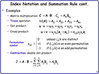
15. 15
Tensor Operations cont.
• Symmetric and skew tensors
– Symmetric
– Skew
– Every tensor can be uniquely decomposed by symmetric and
skew tensors
– Note: W has zero diagonal components and Wij = - Wji
• Properties – Let A be a symmetric tensor
 
 
T
1
2
T
1
2
( )
( )
S T T
W T T


T
T
S S
W W
 
T S W


: 0
: :
A W
A T A S

16. 16
Example
• Displacement gradient can be considered a tensor (rank 2)
  
  
  
  
  
  
 
 

   
  
   

 
 
 
 
1 1 1
1 2 3
2 2 2
1 2 3
3 3 3
1 2 3
u u u
X X X
u u u
X X X
u u u
X X X
u
u
X

   
    

   
    
  
 
    
 
 
 
 
   
 
 
 
 
 
3
1 1 2 1
1 2 1 3 1
3
1 2 2 2
2 1 2 3 2
3 3 3
1 2
3 1 3 2 3
u
u u u u
1 1
X 2 X X 2 X X
u
u u u u
1 1
2 X X X 2 X X
u u u
u u
1 1
2 X X 2 X X X
( ) ( )
sym( ) ( ) ( )
( ) ( )
u

  
   

  
   
 
 
   
 
 
 
 
    
 
 
   
 
 
3
1 2 1
2 1 3 1
3
1 2 2
2 1 3 2
3 3
1 2
3 1 3 2
u
u u u
1 1
2 X X 2 X X
u
u u u
1 1
2 X X 2 X X
u u
u u
1 1
2 X X 2 X X
0 ( ) ( )
skew( ) ( ) 0 ( )
( ) ( ) 0
u
Strain tensor
Spin
tensor

17. 17
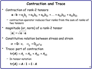
Contraction and Trace
• Contraction of rank-2 tensors
– contraction operator reduces four ranks from the sum of ranks of
two tensors
• magnitude (or, norm) of a rank-2 tensor
• Constitutive relation between stress and strain
• Trace: part of contraction
– In tensor notation
     

ij ij 11 11 12 12 32 32 33 33
: a b a b a b a b a b
a b
 :
a a a
   
  ij ijkl kl
: , D
D
   
ii 11 22 33
tr( ) A A A A
A
 
tr( ) : :
A A 1 1 A

18. 18
Orthogonal Tensor
• In two different coord.
• Direction cosines
• Change basis
  * *
i i j j
u u
u e e
*
ij i j
[ ] [ ]
   
e e
 *
i ij j

e e
 
 
* *
j j i i
*
i ij j
u u
u
u e e
e
 *
j ij i
u u
T *
u u
e1
*
e2
*
e3
*
e1
e2
e3
We can also show
 
 
* *
j ij i
e e u u
  
    
T * T T
( ) ( )
u u u u
  
   
T T
det( ) 1
1
Orthogonal tensor


 
1 T
  
 
* T *
ij ik kl jl
, T T
T T
Rank-2 tensor transformation

19. 19
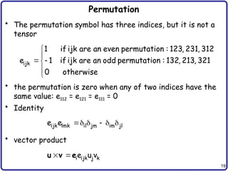
Permutation
• The permutation symbol has three indices, but it is not a
tensor
• the permutation is zero when any of two indices have the
same value: e112 = e121 = e111 = 0
• Identity
• vector product


 



ijk
1 if ijk are an even permutation : 123, 231, 312
e 1 if ijk are an odd permutation : 132, 213, 321
0 otherwise
    
ijk lmk il jm im jl
e e
  i ijk j k
e u v
u v e

20. 20
Dual Vector
• For any skew tensor W and a vector u
– Wu and u are orthogonal
• Let
• Then,
     
T
0
u Wu u W u u Wu

ij ijk k
W e w

   
 
 
    
 
 
 
  
   
12 13 23
12 23 13
13 23 12
0 W W W
W 0 W W
W W 0 W
W w
 
ij j ijk k j ikj k j
W u e w u e w u
 
Wu w u
Dual vector of skew tensor W
 1
i ijk jk
2
w e W

21. 21
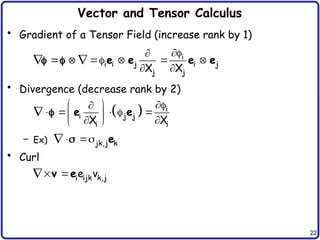
Vector and Tensor Calculus
• Gradient
– Gradient is considered a vector
– We will often use a simplified notation:
• Laplace operator
• Gradient of a scalar field f(X): vector
( )
 
X

 
  
 
i
i
X
e
X
,
i
i j
j
v
v
X



 
 
   
    
 
   
   
   
2
i j
i j j j
X X X X
e e

 

i
i
( )
X
X e
  
 
  
2 2 2
2 2 2
1 2 3
X X X

22. 22
Vector and Tensor Calculus
• Gradient of a Tensor Field (increase rank by 1)
• Divergence (decrease rank by 2)
– Ex)
• Curl


       
 
  i
i i j i j
j j
X X
e e e e
  
 

    
 
 
 
 i
i j j
i i
X X
e e
 
 jk,j k
e
  i ijk k,j
e v
v e

23. 23
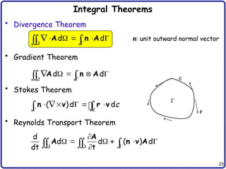
Integral Theorems
• Divergence Theorem
• Gradient Theorem
• Stokes Theorem
• Reynolds Transport Theorem
d d
 
    

 
A n A
d d
 
    

 
A n A
( )d d
c
c

    
 
n v r v

G
c
r
d
d d ( ) d
dt t
  

     


 
 
A
A n v A
n: unit outward normal vector

24. 24
Integration-by-Parts
• u(x) and v(x) are continuously differentiable functions
• 1D
• 2D, 3D
• For a vector field v(x)
• Green’s identity
b b
b
a
a a
u(x)v (x)dx u(x)v(x) u (x)v(x)dx
 
 
 
 
 
i
i i
u v
vd uvn d u d
x x
  
 
    
 
  
u d u( )d u d
  
        
  
v v n v
2
u vd u v d u vd
  
         
  
n

25. 25
Example: Divergence Theorem
• S: unit sphere (x2
+ y2
+ z2
= 1), F = 2xi + y2
j + z2
k
• Integrate d
S
S

F n
S
dS d
2 (1 y z)d
2 d 2 yd 2 zd
2 d
8
3


  

   
   
     
 


 




 
 



F n F

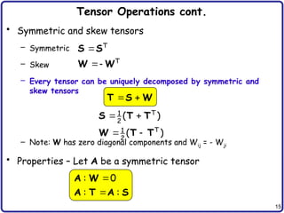
26. 26
Quiz
• A symmetric rank four tensor is defined by
where 1 = [dij] is a unit tensor of rank-two and
is a symmetric unit tensor of rank-
four. When E is an arbitrary symmetric rank-two tensor,
calculate S = D:E in terms of E.
   
2
D 1 1 I
     
1
ik jl il jk
2
[ ]
I

27. 27
STRESS AND STRAIN
1.3

28. 28
Surface Traction (Stress)
• Surface traction (Stress)
– The entire body is in equilibrium with
external forces (f1 ~ f6)
– The imaginary cut body is in equilibrium due
to external forces (f1, f2, f3) and internal
forces
– Internal force acting at a point P
on a plane whose unit normal is n:
– The surface traction depends on the unit
normal direction n.
– Surface traction will change as n changes.
– unit = force per unit area (pressure)
f1
f2
f3
f4
f6
f5
y
z
F
n
f1
f2
f3
P
A
x
( )
A 0
lim
A
 



n F
t
( )
1 1 2 2 3 3
t t t
  
n
t e e e

29. 29
Cartesian Stress Components
• Surface traction changes according to the direction of
the surface.
• Impossible to store stress information for all directions.
• Let’s store surface traction parallel to the three
coordinate directions.
• Surface traction in other directions can be calculated
from them.
• Consider the x-face of an infinitesimal cube
s11
s12
s13
x y
z
Dx
Dy
Dz
DF
(x) (x) (x)
(x)
1 2 3
1 2 3
t t t
 
t e e e
+
(x)
11 1 12 2 13 3
   
t e e e
+
Normal
stress
Shear
stress

30. 30
Stress Tensor
– First index is the face and the second index is its direction
– When two indices are the same, normal stress, otherwise shear
stress.
– Continuation for other surfaces.
– Total nine components
– Same stress components are defined for the negative planes.
• Rank-2 Stress Tensor
• Sign convention
s11 s22
s33
s12
s13
s21
s23
s31
s32
x y
z
Dx
Dy
Dz
ij i j
 
e e

11 x
12 y
sgn( ) sgn( ) sgn( F )
sgn( ) sgn( ) sgn( F )
   
   
n
n

31. 31
Symmetry of Stress Tensor
– Stress tensor should be symmetric
9 components 6 components
– Equilibrium of the angular moment
– Similarly for all three directions:
– Let’s use vector notation:
12
21
x
y
12
21
O
l
l
A B
C D
12 21
12 21
M l( ) 0
    
  

11 12 13
ij 12 22 23
13 23 33
[ ]
  
 
 
    
 
 
  
 
11
22
33
12
23
13
{ }

 
 

 
 

 

 
 

 

 

12 21 23 32 13 31
, ,
     
Cartesian components
of stress tensor

32. 32
Stress in Arbitrary Plane
– If Cartesian stress components are known, it is possible to
determine the surface traction acting on any plane.
– Consider a plane whose normal is n.
– Surface area (ABC = A)
– The surface traction
– Force balance
3 1 2
PAB An ; PBC An ; PAC An
     
x
y
z
B
A
C
s33
s31
s32
s22
s23
s21
s11
s13
s12
t(n)
n
P
( ) ( ) ( )
( )
1 2 3
1 2 3
t t t
  
n n n
n
t e e e
( )
1 11 1 21 2 31 3
1
F t A An An An 0
       
 n
( )
11 1 21 2 31 3
1
t n n n
    
n

33. 33
Cauchy’s Lemma
• All three-directions
• Tensor notation
– stress tensor; completely characterize the state of stress at a
point
• Cauchy’s Lemma
– the surface tractions acting on opposite sides of the same surface
are equal in magnitude and opposite in direction
( )
12 1 22 2 32 3
2
( )
13 1 23 2 33 3
3
t n n n
t n n n
    
    
n
n
( )
11 1 21 2 31 3
1
t n n n
    
n
( ) ( )
    
n n
t n t n
 


( ) ( )
n n
t t

34. 34
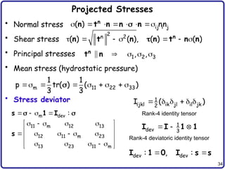
Projected Stresses
• Normal stress
• Shear stress
• Principal stresses
• Mean stress (hydrostatic pressure)
• Stress deviator
ij i j
( ) nn
      
n
n t n n n

      

2
n 2
( ) ( ), ( ) ( )
n
n t n n t n n
   
 1 2 3
, ,
n
t n
   
    
 
 
     
 
 
    
 
 
m dev
11 m 12 13
12 11 m 23
13 23 11 m
:
s 1 I
s
m 11 22 33
1 1
p tr( ) ( )
3 3
       

1
dev 3
  
I I 1 1
1
ijkl ik jl il jk
2
I ( )
     
Rank-4 identity tensor
Rank-4 deviatoric identity tensor
 
dev dev
: , :
I 1 0 I s s

35. 35
Principal Stresses
• Normal & shear stress change as n changes
– Is there a plane on which the normal (or shear)stress becomes the
maximum?
• There are at least three mutually perpendicular planes
on which the normal stress attains an extremum
– Shear stresses are zero on these planes  Principal directions
– Traction t(n)
is parallel to surface normal n
• Eigenvalue problem

( )
n
n
t n  
 n
n n
Principal
stress
Principal
direction
   
 n
[ ]
1 n 0
    
     
   
 
     
   
 
   
 
    
     
11 n 12 13 1
12 22 n 23 2
13 23 33 n 3
n 0
n 0
n 0

36. 36
Eigenvalue Problem for Principal Stresses
• The eigenvalue problem has non-trivial solution if and only
if the determinant is zero:
• The above equation becomes a cubic equation:
• Three roots are principal stresses
    
     
    
11 n 12 13
12 22 n 23
13 23 33 n
0
      
3 2
n 1 n 2 n 3
I I I 0
    
             
                

1 11 22 33
2 2 2
2 11 22 22 33 33 11 12 23 13
2 2 2
3 11 22 33 12 23 13 11 23 22 13 33 12
I
I
I 2
  
1 2 3

37. 37
Principal Directions
• Stress Invariants: I1, I2, I3
– independent of the coordinate system
• Principal directions
– Substitute each principal stress to the eigenvalue problem to get n
– Since the determinant is zero, an infinite number of solutions
exist
– Among them, choose the one with a unit magnitude
• Principal directions are mutually perpendicular
    
2
i i 2 i 2 i 2
1 2 3
(n ) (n ) (n ) 1, i 1,2,3
n
  
j
i
0, i j
n n

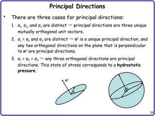
38. 38
Principal Directions
• There are three cases for principal directions:
1. σ1, σ2, and σ3 are distinct  principal directions are three unique
mutually orthogonal unit vectors.
2. σ1 = σ2 and σ3 are distinct  n3
is a unique principal direction, and
any two orthogonal directions on the plane that is perpendicular
to n3
are principal directions.
3. σ1 = σ2 = σ3  any three orthogonal directions are principal
directions. This state of stress corresponds to a hydrostatic
pressure.
n3

39. 39
Strains (Simple Version)
– Strain is defined as the elongation per unit length
– Tensile (normal) strains in x1- and x2-directions
P P
Dx1 Du1
Dx2
Du2
 
 
 
  
 
 
  
 
1
2
1 1
11
x 0 1 1
2 2
22
x 0 2 2
u u
lim
x x
u u
lim
x x
Textbook has different, but
more rigorous derivations

40. 40
Shear Strain
– Shear strain is the tangent of the change in angle between two
originally perpendicular axes
– Shear strain (change of angle)
P
Du1
Du2
q2
q1
p/2 – g12

  


  

2
1 1
1
1
2 2
2
u
~ tan
x
u
~ tan
x
   
   
       
   
1 2
2 1 2 1
12 1 2
x 0 x 0
1 2 1 2
u u u u
lim lim
x x x x
 
 
    
 
 
 
2 1
12 12
1 2
u u
1 1
2 2 x x
Dx1
Dx2

41. 41
Strains (Rigorous Version)
• Strain: a measure of deformation
– Normal strain: change in length of a line segment
– Shear strain: change in angle between two perpendicular line
segments
• Displacement of P = (u1, u2, u3)
• Displacement of Q & R

  


  


  

R 1
1 1 2
2
R 2
2 2 2
2
R 3
3 3 2
2
u
u u x
x
u
u u x
x
u
u u x
x

  


  


  

Q 1
1 1
1
1
Q 2
2 1
2
1
Q 3
3 1
3
1
u
u u x
x
u
u u x
x
u
u u x
x
P(x1,x2,x3) Q
R P'(x1+u1, x2+u2, x3+u3)
Q'
R'
x1
x2
x3
Dx1
Dx2

42. 42
Displacement Field
• Coordinates of P, Q, and R before and after deformation
• Length of the line segment P'Q'
 
 
       
     

 
           
  
     
1 2 3
1 1 2 3
1 1 2 3
P P P
1 1 2 2 3 3 1 1 2 2 3 3
Q Q Q
1 1 2 3
1 2 3
3
1 2
1 1 1 1 2 2 1 3 3 1
1 1 1
R R R
1 1 2 2 2 3 3
P : (x ,x ,x )
Q : (x x ,x ,x )
R : (x ,x x ,x )
P : (x u ,x u ,x u ) (x u ,x u ,x u )
Q : (x x u ,x u ,x u )
u
u u
(x x u x ,x u x ,x u x )
x x x
R : (x u ,x x u ,x u

 
           
  
3
1 2
1 1 2 2 2 2 2 3 3 2
2 2 2
)
u
u u
(x u x ,x x u x ,x u x )
x x x
     
  
  
       
2 2 2
Q Q Q
P P P
1 2 3
1 2 3
P Q x x x x x x

43. 43
Deformation Field
• Length of the line segment P'Q'
• Linear normal strain

 
 
 

 
1
1
u
x 1
x
Linear Nonlinear Ignore H.O.T. when displacement
gradients are small
  

  

1
11
1
u
P Q PQ
PQ x


   
 
3
2
22 33
2 3
u
u
,
x x

   
   
       
   
  
     
 

    
   
 
      
   
 
   
     
 
 

    
   
 
      
   
 
   
     
 
2
2 2
3
1 2
1
1 1 1
1/2
2
2 2
3
1 1 2
1
1 1 1 1
2
2 2
3
1 1 2
1
1 1 1 1
u
u u
P Q x 1
x x x
u
u u u
x 1 2
x x x x
u
u u u
1 1 1
x 1
x 2 x 2 x 2 x

44. 44
Deformation Field
• Shear strain gxy
– change in angle between two lines originally parallel to x– and y–
axes
Engineering shear strain

 
  
 
Q Q
2 2 2
1
1 1
x x u
x x

 
  
 
R R
1 1 1
2
2 2
x x u
x x
 
     
 
1 2
12 1 2
2 1
u u
x x


  
 
 
  
 
3
2
23
3 2
3 1
13
1 3
u
u
x x
u u
x x
 
 
  
 
 
 


 
  
 
 
 
 
 
  
 
 
 
1 2
12
2 1
3
2
23
3 2
3 1
13
1 3
u u
1
2 x x
u
u
1
2 x x
u u
1
2 x x
Different notations

 

  
 
 
 
 
j
i
ij
j i
u
u
1
2 x x
  
1
ij i,j j,i
2
(u u )
 
 sym( )
u

45. 45
Strain Tensor
• Strain Tensor
• Cartesian Components
• Vector notation
ij i j
 
e e

11 12 13
ij 12 22 23
13 23 33
[ ]
  
 
 
   
 
 
  
 

11 11
22 22
33 33
12 12
23 23
13 13
{ }
2
2
2
 
   
   
 
   
   
 
 
   
 
   
   
 
   
 
   


46. 46
Volumetric and Deviatoric Strain
• Volumetric strain (from small strain assumption)
• Deviatoric strain
0
V 11 22 33 11 22 33
0
V V
(1 )(1 )(1 ) 1
V

              
V 11 22 33 kk
      
1 1
V ij ij V ij
3 3
e
      
e 1

dev :

e I 
x2
x3
x1
1
e11
e22
e33
1
1
Exercise: Write Idev in matrix-vector notation

47. 47
Stress-Strain Relationship
• Applied Load shape change (strain) stress
• There must be a relation between stress and strain
• Linear Elasticity: Simplest and most commonly used
Proportional
limit
Yield stress
Ultimate
stress
Strain
hardening
Necking
Fracture
s
e
Young’s
modulus

48. 48
Generalized Hooke’s Law
• Linear elastic material
– In general, Dijkl has 81 components
– Due to symmetry in sij, Dijkl = Djikl
– Due to symmetry in ekl, Dijkl = Dijlk
– from definition of strain energy, Dijkl = Dklij
• Isotropic material (no directional dependence)
– Most general 4-th order isotropic tensor
– Have only two independent coefficients
(Lame’s constants: l and m)
21 independent coeff
ijkl ij kl ik jl il jk
ij kl ik jl il jk
D
( )
       
        
ij ijkl kl
: , D
   
D
 
2
   
D 1 1 I

49. 49
Generalized Hooke’s Law cont.
• Stress-strain relation
– Volumetric strain:
– Off-diagonal part:
– Bulk modulus K: relation b/w volumetric stress & strain
– Substitute so that we can separate volumetric part
• Total deform. = volumetric + deviatoric deform.
ij ijkl kl ij kl ik jl il jk kl kk ij ij
D [ ( )] 2
                 
kk 11 22 33 v
      
12 12 12
2
    m is the shear modulus
1 m jj kk jj jj kk
I 3 2 (3 2 )
           
       
2
m kk v
3
p ( ) K
Bulk modulus
2
3
K
   

50. 50
Generalized Hooke’s Law cont.
• Stress-strain relation cont.
2
ij kk ij ij
3
2
kk ij ij kk ij
3
1
ij kl kl ik jl ij kl kl
3
ij kl dev ijkl kl
(K ) 2
K 2
K 2 [ ]
K 2 (I )
       
       
           
 
     
 
dev
σ K 2 : ε
    
 
 
1 1 I
Deviatoric part
Volumetric part
v
m
σ K 2
σ
    
  
1 e
1 s
dev :

e I 
Deviatoric strain
Important for plasticity; plastic deformation only occurs in deviatoric part
volumetric part is always elastic
dev :

s I 
Deviatoric stress

51. 51
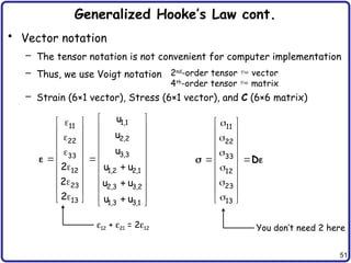
Generalized Hooke’s Law cont.
• Vector notation
– The tensor notation is not convenient for computer implementation
– Thus, we use Voigt notation
– Strain (6×1 vector), Stress (6×1 vector), and C (6×6 matrix)
2nd
-order tensor  vector
4th
-order tensor  matrix
1,1
11
2,2
22
3,3
33
12 1,2 2,1
23 2,3 3,2
13 1,3 3,1
u
u
u
2 u u
2 u u
2 u u
 

 
 
 
  
 
 
 

 
 
 
 
 
 
 
 
 
 
 
  
  
 

11
22
33
12
23
13

 
 

 
 

 
 

 
 

 

 
D
 
e12 + e21 = 2e12 You don’t need 2 here

52. 52
3D Solid Element cont.
• Elasticity matrix
• Relation b/w
Lame’s constants
and Young’s modulus
and Poisson’s ratio
(3 2 )
, E
2( )
E E
,
(1 )(1 2 ) 2(1 )
    
  
     

   
     
dev
K 2
   
D 1 1 I
2 0 0 0
2 0 0 0
2 0 0 0
0 0 0 0 0
0 0 0 0 0
0 0 0 0 0
    
 
 
    
 
 
    
 

 
 

 

 
D
1
1
1
0
0
0
 
 
 
 
 
 
 
 
 
1
2 1 1
3 3 3
1 2 1
3 3 3
1 1 2
3 3 3
dev 1
2
1
2
1
2
0 0 0
0 0 0
0 0 0
0 0 0 0 0
0 0 0 0 0
0 0 0 0 0
 
 
 
 
 
 
 
 

 
 
 
 
 
I
Textbook has a definition of D in terms of E and n

53. 53
Plane Stress
• Thin plate–like components parallel to the xy–plane
• The plate is subjected to forces in its in-plane only
• s13 = s23 = s33 = 0
• e13 = e23 = 0, but e33 ≠ 0
• e33 can be calculated from the condition of s33 = 0:
11 11
22 22
2
1
12 12
2
1 0
E
{ } 1 0
1
0 0 (1 )
 
  
   
   
 
    
   
 
 
   
 
   
   
 


    
 
33 11 22
( )
1

54. 54
Plane Strain
• Strains with a z subscript are all zero: e13 = e23 = e33 = 0
• Deformation in the z–direction is constrained, (i.e., u3 = 0)
• can be used if the structure is infinitely long in the z–
direction
• s13 = s23 = 0, but s33 ≠ 0
• s33 can be calculated from the condition of e33 = 0:
11 11
22 22
1
12 12
2
1 0
E
{ } 1 0
(1 )(1 2 )
0 0
 
    
   
   
 
      
   
 
   
   
 
   
   
 

 
33 11 22
E
(1 )(1 2 )

    
   

55. 55
MECHANICS OF
CONTINUOUS BODIES
1.4

56. 56
Governing Equations for Equilibrium
• Governing differential equations for structural equilibrium
– Three laws of mechanics: conservation of mass, conservation of
linear momentum and conservation of angular momentum
• Boundary-valued problem: satisfied at every point in W
– Governing D.E. + Boundary conditions
– Solutions: C2
–continuous for truss & solid, C4
–continuous for beam
– Unnecessarily requirements for higher-order continuity
• Energy-based method
– For conservative system, structural equilibrium when the potential
energy has its minimum: Principle of minimum potential energy
– If the solution of BVP exists, then that solution is the minimizing
solution of the potential energy
– When no solution exists in BVP, PMPE may have a natural solution
• Principle of virtual work
– Equilibrium of the work done by both internal and external forces
with small arbitrary virtual displacements

57. 57
Balance of Linear Momentum
• Balance of linear momentum
• Stress tensor (rank 2):
• Surface traction
• Cauchy’s Lemma
  
     

  

b
d d d
n
f t a
ij i j
 
e e

11 12 13
ij 21 22 23
31 32 33
  
 
 
 
    
   
 
  
 
 
n
t n 


n n
t t

   
n n
t n t n
 
W
G
n
tn
X1
X2
X3
e1 e2
e3
X
fb
: body force
tn
: surface traction
0 for static problem

58. 58
Balance of Linear Momentum cont
• Balance of linear momentum
– For a static problem
• Balance of angular momentum
  
        

  

 
b
( )d d d
f a n

     

  b
[ ( )]d 0
f a
    
 b
( ) 0
f a
     
 b b
ij,i j
0 f 0
f
  
        

  

b
d d d
n
x f x t x a
T
ij ji
  
 
Divergence Theorem

59. 59
Boundary-Valued Problem
• We want to determine the state of a body in equilibrium
• The equilibrium state (solution) of the body must satisfy
– local momentum balance equation
– boundary conditions
• Strong form of BVP
– Given body force fb
, and traction t
on the boundary, find u such that
and
• Solution space
h
s
on essential BC
on natural BC
 
  
u 0
t n 
  
 b
0
f (1)
(2)
(3)
W
G
n
t
X1
X2
X3
e1 e2
e3
X
fb
 
2 3 h s
A
D [C ( )] | 0 on , on
         
u u x n t x


60. 60
Boundary-Valued Problem cont.
• How to solve BVP
– To solve the strong form, we want to construct trial solutions that
automatically satisfy a part of BVP and find the solution that
satisfy remaining conditions.
– Statically admissible stress field: satisfy (1) and (3)
– Kinematically admissible displacement field: satisfy (2) and have
piecewise continuous first partial derivative
– Admissible stress field is difficult to construct. Thus, admissible
displacement field is used often

61. 61
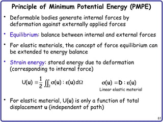
Principle of Minimum Potential Energy (PMPE)
• Deformable bodies generate internal forces by
deformation against externally applied forces
• Equilibrium: balance between internal and external forces
• For elastic materials, the concept of force equilibrium can
be extended to energy balance
• Strain energy: stored energy due to deformation
(corresponding to internal force)
• For elastic material, U(u) is only a function of total
displacement u (independent of path)
1
U( ) ( ) : ( )d
2 
 


u u u
  ( ) : ( )

u D u
 
Linear elastic material

62. 62
PMPE cont.
• Work done by applied loads (conservative loads)
• U(u) is a quadratic function of u, while W(u) is a linear
function of u.
• Potential energy
s
b
W( ) d d .
 
     

 
u u f u t
Gh
Gg
W
u1 u2
u3
x1
x2
x3
fs
fb
s
b
( ) U( ) W( )
1
( ) : ( )d d d .
2   
  
       

 
 
u u u
u u u f u t
 

63. 63
PMPE cont.
• PMPE: for all displacements that satisfy the boundary
conditions, known as kinematically admissible
displacements, those which satisfy the boundary-valued
problem make the total potential energy stationary on DA
• But, the potential energy is well defined in the space of
kinematically admissible displacements
• No need to satisfy traction BC (it is a part of potential)
• Less requirement on continuity
• The solution is called a generalized (natural) solution
 
1 3 h
[H ( )] | 0 on ,
     
u u x
Z
H1
: first-order derivatives are integrable

64. 64
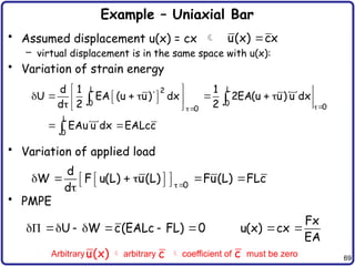
Example – Uniaxial Bar
• Strong form
• Integrate twice:
• Apply two BCs:
• PMPE with assumed solution u(x) = c1x + c2
• To satisfy KAD space, u(0) = 0,  u(x) = c1x
• Potential energy:
L
F
x
EAu 0 x [0,L]
u 0 x 0
EAu (L) F x L

  
 
  
1 2
EAu(x) c x c
 
Fx
u(x)
EA

L 2 2
1
0
1
1
U EA(u ) dx EALc
2
W Fu(L) FLc

 
 

1
1 1
d d
(U W) EALc FL 0
dc dc

     1
F Fx
c u(x)
EA EA
  
Solution of BVP

65. 65
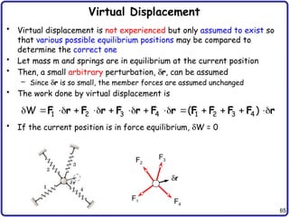
Virtual Displacement
• Virtual displacement is not experienced but only assumed to exist so
that various possible equilibrium positions may be compared to
determine the correct one
• Let mass m and springs are in equilibrium at the current position
• Then, a small arbitrary perturbation, dr, can be assumed
– Since dr is so small, the member forces are assumed unchanged
• The work done by virtual displacement is
• If the current position is in force equilibrium, dW = 0
             
1 2 3 4 1 2 3 4
W ( )
F r F r F r F r F F F F r
F1
F2
F3
F4
dr

66. 66
Virtual Displacement Field
• Virtual displacement (Space Z)
– Small arbitrary perturbation (variation) of real displacement
– Let ū be the virtual displacement, then u + ū must be kinematically
admissible, too
– Then, ū must satisfy homogeneous displacement BC
– Space Z only includes homogeneous
essential BCs
• Property of variation
    
u u u u
V Z

 
h
1 3
[H ( )] , 0

   
u u u
Z
u
ū
In the literature, du is often used instead of ū
d d( )
dx dx

 
 
 
 
u u
0
0
1 d
lim [( ) ( )] ( ) .
d


         
 
u u u u u
  

67. 67
PMPE As a Variation
• Necessary condition for minimum PE
– Stationary condition <--> first variation = 0
• Variation of strain energy
0
0
1 d
( ; ) lim [ ( ) ( )] ( ) 0
d


           
 
u u u u u u u
 Z
for all u
0
d
d 
    
   
  
   
   
   
u u u u
x x x
( ) ( )
  
u u
   :
 D
 
1
2
U( ; ) ( ) : : ( ) ( ) : : ( ) d
( ) : : ( )d
a( , )


   
 
 
 





u u u D u u D u
u D u
u u
   
 
Energy bilinear form

68. 68
PMPE As a Variation cont.
• Variation of work done by applied loads
• Thus, PMPE becomes
– Load form is linear with respect to ū
– Energy form a(u, ū) is symmetric, bilinear w.r.t. u and ū
– Different problems have different a(u, ū) and , but they share
the same property
• How can we satisfy “for all ū  ” requirement?
Can we test an infinite number of ū?
s
b
W( ; ) d d ( )
 
       

 
u u u f u t u

a( , ) ( ),
  
u u u u Z

( )
u

( )
u

( ; ) U( ; ) W( ; ) 0
    
u u u u u u
Load linear form

69. 69
Example – Uniaxial Bar
• Assumed displacement u(x) = cx 
– virtual displacement is in the same space with u(x):
• Variation of strain energy
• Variation of applied load
• PMPE
u(x) cx

L L
2
0 0 0
0
L
0
d 1 1
U EA (u u) dx 2EA(u u) u dx
d 2 2
EAu u dx EALcc


 
  
      
 
 
 
  
 
 
 

0
d
W F u(L) u(L) Fu(L) FLc
d 
     
   
   

U W c(EALc FL) 0
      
Fx
u(x) cx
EA
 
Arbitrary  arbitrary  coefficient of must be zero
u(x) c c

70. 70
Principle of Virtual Work
• Instead of solving the strong form directly, we want to
solve the equation with relaxed requirement (weak form)
• Virtual work – Work resulting from real forces acting
through a virtual displacement
• Principle of virtual work – when a system is in equilibrium,
the forces applied to the system will not produce any
virtual work for arbitrary virtual displacements
– Balance of linear momentum is force equilibrium
– Thus, the virtual work can be obtained by multiplying the force
equilibrium equation with a virtual displacement
– If the above virtual work becomes zero for arbitrary ū, then it
satisfies the original equilibrium equation in a weak sense
b
0
   
f


    

  b
W ( ) d
f u

71. 71
Principle of Virtual Work cont
• PVW
– Integration-by-parts
– Divergence Thm
– The boundary is decomposed by

     


b
ij,i j j
( f )u d 0 u Z
 
    

 

b
ij,i j j j
u d f u d
 
 
      
 

 

b
ij j ,i ij j,i j j
( u ) u d f u d
  
       
 
 

b
i ij j ij j,i j j
n u d u d f u d
h s
j i ij j
u 0 on and n t on
    
h s
   
S
b
j j ij j,i j j
t u d u d f u d
0
  
      
  
 
 

u 

72. 72
Principle of Virtual Work cont
• Since sij is symmetric
• Weak Form of BVP
Internal virtual work = external virtual work
Starting point of FEM
• Symbolic expression
– Energy form:
– Load form:
  
        

 
 s
b
ij ij j j j j
d f u d t u d u Z
a( , ) ( )
  
u u u u Z

a( , ) : d

 


u u  
s
b
( ) d d
 
      

 
u u f u t

ij j,i ij j,i ij ij
u sym(u )
   
j
i
i,j ij
j i
u
u
1
sym(u )
2 X X

 

  
 
 
 
 
[ ]{ } { }

K d F
FE equation

73. 73
Example – Heat Transfer Problem
• Steady-State Differential Equation
• Boundary conditions
• Space of kinematically admissible temperature
• Multiply by virtual temperature, integrate by part, and
apply boundary conditions
Q
domain A
Sq
ST
qn
T = T0
n = {nx, ny}T
y
x
T
T
k Q 0
k
y
x y
x

   

    
   

 
 
  
0 T
n x x y y q
T T on S
dT dT
q n k n k on S
dx dy




 


 
1
T
T H ( ) T( ) 0, S
     
x x
Z
q
x y n q
S
T T T T
k k d TQd Tq dS , T
x x y y
 
 
   
      
 
   
 
   Z

74. 74
Example – Beam Problem
• Governing DE
• Boundary conditions for cantilevered beam
• Space of kinematically admissible displacement
• Integrate-by-part twice, and apply BCs
4
4
d v
EI f(x), x [0,L]
dx
 
2 3
2 3
dv d v d v
v(0) (0) (L) (L) 0
dx dx dx
   
f(x)
x L
2 dv
v H [0,L] v(0) (0) 0
dx
 
   
 
 
Z
2 2
L L
2 2
0 0
d v d v
EI dx fv dx, v
dx dx
  
  Z

75. 75
Difference b/w Strong and Weak Solutions
• The solution of the strong form needs to be twice
differentiable
• The solution of the weak form requires the first-order
derivatives are integrable  bigger solution space than
that of the strong form
• If the strong form has a solution, it is the solution of the
weak form
• If the strong form does not have a solution, the weak
form may have a natural solution
F
y
x
T
T k Q 0
k
y
x y
x

   

    
   

 
 
  
x y
T T T T
k k d
x x y y

 
   
 
 
   
 


76. 76
FINITE ELEMENT METHOD
1.5

77. 77
Finite Element Approximation
• Difficult to solve a variational equation analytically
• Approximate solution
– Linear combination of trial functions
– Smoothness & accuracy depend on
the choice of trial functions
– If the approximate solution is expressed in the entire domain, it is
difficult to satisfy kinematically admissible conditions
• Finite element approximation
– Approximate solution in simple sub-domains (elements)
– Simple trial functions (low-order polynomials) within an element
– Kinematically admissible conditions only for elements on the
boundary
n
i i
i 1
u(x) c (x)

 

Exact solution
Approximate
solution
x
u(x)
Finite elements
Nodes
Piecewise-
linear
approximation

78. 78
Finite Elements
• Types of finite elements
1D 2D 3D
• Variational equation is imposed on each element.
One element
1 0.1 0.2 1
0 0 0.1 0.9
dx dx dx dx
   
   

Linear
Quadratic

79. 79
Trial Solution
– Solution within an element is approximated using simple
polynomials.
– i-th element is composed of two nodes: xi and xi+1. Since two
unknowns are involved, linear polynomial can be used:
– The unknown coefficients, a0 and a1, will be expressed in terms of
nodal solutions u(xi) and u(xi+1).
1 2 3 n 1 n+1
n
1 2 n 1 n
xi xi+1
i
l
0 1 i i 1
u(x) a a x, x x x
   

80. 80
Trial Solution cont.
– Substitute two nodal values
– Express a0 and a1 in terms of ui and ui+1. Then, the solution is
approximated by
– Solution for Element e:
–
i i 0 1 i
i 1 i 1 0 1 i 1
u(x ) u a a x
u(x ) u a a x
  
  


  

1 2
i 1 i
i i 1
(e) (e)
N (x) N (x)
x x x x
u(x) u u
L L


 
 
     
1 i 2 i 1 i i 1
u(x) N (x)u N (x)u , x x x
 
   

81. 81
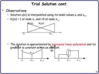
Trial Solution cont.
• Observations
– Solution u(x) is interpolated using its nodal values ui and ui+1.
– N1(x) = 1 at node xi, and =0 at node xi+1.
– The solution is approximated by piecewise linear polynomial and its
gradient is constant within an element.
N1(x) N2(x)
xi xi+1
xi xi+1 xi+2 xi xi+1 xi+2
ui
ui+1
ui+2 du
dx
u

82. 82
1D Finite Elements
• 1D BVP
• Use PVW
• Integration-by-parts
– This variational equation also satisfies at individual element level
   
 


 

2
2
d u
p(x) 0, 0 x 1
dx
u(0) 0
Boundary conditions
du
(1) 0
dx
2
1
2
0
d u
p u dx 0
dx
 
 
 
 
  
(1)
u H [0,1] u(0) 0
  
Z
Space of kinematically
admissible displacements
1
1 1
0 0
0
du du du
u dx pu dx
dx dx dx
 
 
j j
i i
x x
x x
du du
dx pu dx
dx dx
  
  u 
(1)

83. 83
1D Interpolation Functions
• Finite element approximation for one element (e) at a time
• Satisfies interpolation condition
• Interpolation of displacement variation (same with u)
• Derivative of u(x): differentiating interpolation functions
(e) (e) (e)
i 1 i 1 2
u (x) uN (x) u N (x)

   
N d
i
(e) (e)
1 2
i 1
u
N N
u
 
  
   
 
d N
(e)
i i
(e)
i 1 i 1
u (x ) u
u (x ) u
 


(e) (e) (e)
i 1 i 1 2
u (x) uN (x) u N (x)

   
N d
(e)
i i (e) (e)
1 2
(e) (e)
i 1 i 1
u u
dN dN
du 1 1
dx dx dx u u
L L
 
   
   
    
   
   
 
     
B d

84. 84
Element-Level Variational Equation
• Approximate variational equation (1) for element (e)
– Must satisfied for all
– If element (e) is not on the boundary, can be arbitrary
• Element-level variational equation
j j
i i
i
x x
(e)T (e)T (e) (e) (e)T (e)T (e)T
x x
i 1
du
(x )
dx
dx p(x)dx
du
(x )
dx 
 

 
     
 
   

 
 
d B B d d N d
(e)
u (x)  Z
(e)
d
j j
i i
i
x x
(e)T (e) (e) (e)T
x x
i 1
du
(x )
dx
dx p(x)dx
du
(x )
dx 
 

 
     
 
   

 
 
B B d N
 
i
(e) (e) (e)
i 1
du
(x )
dx
[ ]{ }
du
(x )
dx 
 

 
   
 

 
k d f
2x2 matrix 2x1 vector

85. 85
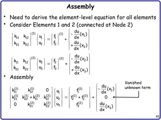
Assembly
• Need to derive the element-level equation for all elements
• Consider Elements 1 and 2 (connected at Node 2)
• Assembly
(1) (1)
1
11 12 1 1
2 2
21 22
2
du
(x )
k k u f dx
u f du
k k (x )
dx
 

 
     
 
     
 
   
   

 
(2) (2)
2
2 2
11 12
3 3
21 22
3
du
(x )
u f
k k dx
u f du
k k
(x )
dx
 

 
     
 
     
 
   
   

 
(1) (1) (1)
1
11 12 1
1
(1) (1) (2) (2) (1) (2)
2
21 22 11 12 2 2
(2) (2) (2)
3
21 22 3
3
du
(x )
k k 0 f
u dx
k k k k u f f 0
u du
0 k k f (x )
dx
 

     
 
     
   
   
       
       
 
     
   
 
Vanished
unknown term

86. 86
Assembly cont.
• Assembly of NE elements (ND = NE + 1)
• Coefficient matrix [K] is singular; it will become non-
singular after applying boundary conditions
 
 
   
E E
E
D
D
D D
(1) (1) (1)
11 12 1
1
(1) (1) (2) (2) (1) (2)
21 22 11 12 2 2
2
(2) (2) (2) (2) (3)
3
221 22 11 3 3
N (N )
(N )
N N
21 22 N 1 N 1
N N
k k 0 0 f
u
k k k k 0 f f
u
u
0 k k k 0 f f
u f
0 0 0 k k
 

 

 
   
 
   
 
 
   
   
   
 
   
     
     
     
   
 
 




     
 
D
1
N
N 1
du
(x )
dx
0
0
du
(x )
dx

 
 
 
 
 
 
 
 
 

 
 

[ ]{ } { }

K d F

87. 87
Example
• Use three equal-length elements
• All elements have the same coefficient matrix
• RHS (p(x) = x)
2
2
d u
x 0, 0 x 1 u(0) 0, u(1) 0
dx
     
(e)
(e)
2 2
1 1 3 3
1
, (e 1,2,3)
1 1 3 3
L

 
   
    
   
   
   
k
i 1 i 1
i i
x x
1 i 1
(e)
(e)
x x
2 i
i i 1
(e)
i i 1
N (x) x(x x)
1
{ } p(x) dx dx
N (x) x(x x )
L
x x
3 6
L , (e 1,2,3)
x x
6 3
  



   
 
   

   
 

 
 
 
 
 

 
 
 
f

88. 88
Example cont.
• RHS cont.
• Assembly
• Apply boundary conditions
– Deleting 1st and 4th rows and columns
(3)
(2)
(1)
3
2
1
(3)
(2)
(1)
3
2 4
f
f
f 1 4 7
1 1 1
, ,
54 54 54
2 5 8
f
f
f
 
 
       
     
  
           
     
     
     
1
2
3
4
1
(0)
54
3 3 0 0 2 4
3 3 3 3 0 54 54
0 3 3 3 3 7 5
54 54
0 0 3 3
8
(1)
54
du
dx
u
u
u
u
du
dx
ì ü
ï ï
ï ï
-
ï ï
ï ï
ï ï
ì ü
é ù
- ï ï ï ï
ï ï ï ï
ê ú
ï ï +
ï ï
ï ï
ê ú
- + - ï ï
ï ï ï ï
ê ú =
í ý í ý
ê ú
ï ï ï ï
- + - ï ï ï ï
ê ú +
ï ï ï ï
ï ï ï ï
ê ú
- ï ï ï ï
ë û
î þ ï ï
ï ï
ï ï
+
ï ï
ï ï
î þ
Element 1
Element 2
Element 3
2
3
u
6 3 1
1
9
u
3 6 2
  
   

   
 

   
 
4
2 81
5
3 81
u
u



89. 89
EXAMPLE cont.
• Approximate solution
• Exact solution
– Three element solutions are poor
– Need more elements
4 1
x, 0 x
27 3
4 1 1 1 2
u(x) x , x
81 27 3 3 3
5 5 2 2
x , x 1
81 27 3 3

 


 

    
  
 

  
   
  
   0
0.02
0.04
0.06
0.08
0 0.2 0.4 0.6 0.8 1
x
u(x)
u-approx.
u-exact
 
2
1
u(x) x 1 x
6
 

90. 90
3D Solid Element
• Isoparametric mapping
– Build interpolation functions on the reference element
– Jacobian: mapping relation between physical and reference elem.
• Interpolation and mapping
(a) Finite Element (b) Reference Element
x
h
z
(1,1,–1)
(1,1,1)
(–1,1,1)
(–1,1,–1)
x1
x2
x3
x4
x5
x6
x7
x8
x2
x1
x3
(1, –1,–1)
(1, –1,1)
(–1, –1,1)
8
I I
I 1
( ) N ( )


u u
 
8
I I
I 1
( ) N ( )


x x
 
I I I I
1
N ( ) (1 )(1 )(1 )
8
      

Same for mapping
and interpolation

91. 91
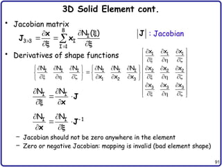
3D Solid Element cont.
• Jacobian matrix
• Derivatives of shape functions
– Jacobian should not be zero anywhere in the element
– Zero or negative Jacobian: mapping is invalid (bad element shape)
8
I
3 3 I
I 1
N ( )




 
 

x
J x

 
1 1 1
I I I I I I 2 2 2
1 2 3
3 3 3
x x x
N N N N N N x x x
x x x
x x x
  
 
 
  
 
        
     

     
        
     
  
 
 
  
 
I I
N N
 
 
 
J
x

1
I I
N N 
 
 
 
J
x 
J : Jacobian

92. 92
3D Solid Element cont.
• Displacement-strain relation
8
I I
I 1
( )


u B u

I,1
I,2
I,3
I
I,2 I,1
I,3 I,2
I,3 I,1
N 0 0
0 N 0
0 0 N
N N 0
0 N N
N 0 N
 
 
 
 
 

 
 
 
 
 
B
8
I I
I 1
( )

 
u B u
 
i
I,i
i
N
N
x




93. 93
3D Solid Element cont.
• Transformation of integration domain
• Energy form
• Load form
• Discrete variational equation
1 1 1
1 1 1
d d d d
   
    


    J
8 8
1 1 1
T T T
I I J J
1 1 1
I 1 J 1
a( , ) d d d { } [ ]{ }
  
 
 
    
 
 
    
u u u B DB J u d k d
8
1 1 1
T b T
I I
1 1 1
I 1
( ) N ( ) d d d { } { }
  

    
   
u u f J d f


T T
h
{ } [ ]{ } { } { }, { }
  
d k d d f d Z

94. 94
Numerical Integration
• For bar and beam, analytical integration is possible
• For plate and solid, analytical integration is difficult, if
not impossible
• Gauss quadrature is most popular in FEM due to simplicity
and accuracy
• 1D Gauss quadrature
– NG: No. of integ. points; xi: integ. point; wi: integ. weight
– xi and wi are chosen so that the integration is exact
for (2*NG – 1)-order polynomial
– Works well for smooth function
– Integration domain is [-1, 1]
NG
1
i i
1
i 1
f( )d f( )


    



95. 95
Numerical Integration cont.
• Multi-dimensions
NG NG
1 1
i j i j
1 1
i 1 j 1
f( , )d d f( , )
 
 
       

 
NG NG NG
1 1 1
i j k i j k
1 1 1
i 1 j 1 k 1
f( , , )d d d f( , , )
  
  
           

  
NG
Integration
Points (xi)
Weights (wi)
1 0.0 2.0
2 .5773502692 1.0
3
.7745966692
0.0
.5555555556
.8888888889
4
.8611363116
.3399810436
.3478546451
.6521451549
5
.9061798459
.5384693101
0.0
.2369268851
.4786286705
.5688888889
x
h
x
h
x
h
(a) 11
(b) 22 (c) 33

96. 96
ELAST3D.m
• A module to solve linear elastic problem using NLFEA.m
• Input variables for ELAST3D.m
Variable Array size Meaning
ETAN (6,6) Elastic stiffness matrix Eq. (1.81)
UPDATE Logical variable If true, save stress values
LTAN Logical variable If true, calculate the global stiffness matrix
NE Integer Total number of elements
NDOF Integer Dimension of problem (3)
XYZ (3,NNODE) Coordinates of all nodes
LE (8,NE) Element connectivity

97. 97
How to Solve Linear Problem in Nonlinear Code
• Linear matrix solver
– Construct stiffness matrix and force vector
– Use LU decomposition to solve for unknown displacement {d}
• Nonlinear solver (iterative solver)
– Assume the solution at iteration n is known, and n+1 is unknown
[ ]{ } { }

K d F {fint
} = {fext
} {f} = {fext
} − {fint
} = {0}
n 1 n
{ } { } { }

  
d d d For linear problem, {dn
} = {0}
n 1 n
{ } { } { } { }
 
 
   
 

 
f
f f d 0
d
n
{ } [ ]{ } [ ]{ } 0
   
F K d K d
[ ]{ } { }
 
K d F Only one iteration!!

98. 98
function ELAST3D(ETAN, UPDATE, LTAN, NE, NDOF, XYZ, LE)
%***********************************************************************
% MAIN PROGRAM COMPUTING GLOBAL STIFFNESS MATRIX AND RESIDUAL FORCE FOR
% ELASTIC MATERIAL MODELS
%***********************************************************************
%%
global DISPTD FORCE GKF SIGMA
%
% Integration points and weights (2-point integration)
XG=[-0.57735026918963D0, 0.57735026918963D0];
WGT=[1.00000000000000D0, 1.00000000000000D0];
%
% Index for history variables (each integration pt)
INTN=0;
%
%LOOP OVER ELEMENTS, THIS IS MAIN LOOP TO COMPUTE K AND F
for IE=1:NE
% Nodal coordinates and incremental displacements
ELXY=XYZ(LE(IE,:),:);
% Local to global mapping
IDOF=zeros(1,24);
for I=1:8
II=(I-1)*NDOF+1;
IDOF(II:II+2)=(LE(IE,I)-1)*NDOF+1:(LE(IE,I)-1)*NDOF+3;
end
DSP=DISPTD(IDOF);
DSP=reshape(DSP,NDOF,8);
%
%LOOP OVER INTEGRATION POINTS
for LX=1:2, for LY=1:2, for LZ=1:2
E1=XG(LX); E2=XG(LY); E3=XG(LZ);
INTN = INTN + 1;
%
% Determinant and shape function derivatives
[~, SHPD, DET] = SHAPEL([E1 E2 E3], ELXY);
FAC=WGT(LX)*WGT(LY)*WGT(LZ)*DET;

99. 99
% Strain
DEPS=DSP*SHPD';
DDEPS=[DEPS(1,1) DEPS(2,2) DEPS(3,3) ...
DEPS(1,2)+DEPS(2,1) DEPS(2,3)+DEPS(3,2) DEPS(1,3)+DEPS(3,1)]';
%
% Stress
STRESS = ETAN*DDEPS;
%
% Update stress
if UPDATE
SIGMA(:,INTN)=STRESS;
continue;
end
%
% Add residual force and stiffness matrix
BM=zeros(6,24);
for I=1:8
COL=(I-1)*3+1:(I-1)*3+3;
BM(:,COL)=[SHPD(1,I) 0 0;
0 SHPD(2,I) 0;
0 0 SHPD(3,I);
SHPD(2,I) SHPD(1,I) 0;
0 SHPD(3,I) SHPD(2,I);
SHPD(3,I) 0 SHPD(1,I)];
end
%
% Residual forces
FORCE(IDOF) = FORCE(IDOF) - FAC*BM'*STRESS;
%
% Tangent stiffness
if LTAN
EKF = BM'*ETAN*BM;
GKF(IDOF,IDOF)=GKF(IDOF,IDOF)+FAC*EKF;
end
end, end, end, end
end

100. 100
function [SF, GDSF, DET] = SHAPEL(XI, ELXY)
%*************************************************************************
% Compute shape function, derivatives, and determinant of hexahedral element
%*************************************************************************
%%
XNODE=[-1 1 1 -1 -1 1 1 -1;
-1 -1 1 1 -1 -1 1 1;
-1 -1 -1 -1 1 1 1 1];
QUAR = 0.125;
SF=zeros(8,1);
DSF=zeros(3,8);
for I=1:8
XP = XNODE(1,I);
YP = XNODE(2,I);
ZP = XNODE(3,I);
%
XI0 = [1+XI(1)*XP 1+XI(2)*YP 1+XI(3)*ZP];
%
SF(I) = QUAR*XI0(1)*XI0(2)*XI0(3);
DSF(1,I) = QUAR*XP*XI0(2)*XI0(3);
DSF(2,I) = QUAR*YP*XI0(1)*XI0(3);
DSF(3,I) = QUAR*ZP*XI0(1)*XI0(2);
end
GJ = DSF*ELXY;
DET = det(GJ);
GJINV=inv(GJ);
GDSF=GJINV*DSF;
end
SF(81): shape functions,
GDSF (38): shape functions derivatives
DET: Jacobian of the mapping

101. 101
One Element Tension Example
%
% One element example
%
% Nodal coordinates
XYZ=[0 0 0;1 0 0;1 1 0;0 1 0;0 0 1;1 0 1;1 1 1;0 1 1];
%
% Element connectivity
LE=[1 2 3 4 5 6 7 8];
%
% External forces [Node, DOF, Value]
EXTFORCE=[5 3 10.0E3; 6 3 10.0E3; 7 3 10.0E3; 8 3 10.0E3];
%
% Prescribed displacements [Node, DOF, Value]
SDISPT=[1 1 0;1 2 0;1 3 0;2 2 0;2 3 0;3 3 0;4 1 0;4 3 0];
%
% Material properties
% MID:0(Linear elastic) PROP=[LAMBDA NU]
MID=0;
PROP=[110.747E3 80.1938E3];
%
% Load increments [Start End Increment InitialFactor FinalFactor]
TIMS=[0.0 1.0 1.0 0.0 1.0]';
%
% Set program parameters
ITRA=30; ATOL=1.0E5; NTOL=6; TOL=1E-6;
%
% Calling main function
NOUT = fopen('output.txt','w');
NLFEA(ITRA, TOL, ATOL, NTOL, TIMS, NOUT, MID, PROP, EXTFORCE, SDISPT, XYZ, LE);
fclose(NOUT);
10kN
x2
x1
x3
1
2
3
4
5
6 7
8
10kN
10kN
10kN

102. 102
One Element Output
Time Time step Iter Residual
1.00000 1.000e+00 2 5.45697e-12
TIME = 1.000e+00
Nodal Displacements
Node U1 U2 U3
1 0.000e+00 0.000e+00 0.000e+00
2 -5.607e-08 0.000e+00 0.000e+00
3 -5.607e-08 -5.607e-08 0.000e+00
4 0.000e+00 -5.607e-08 0.000e+00
5 -5.494e-23 1.830e-23 1.933e-07
6 -5.607e-08 4.061e-23 1.933e-07
7 -5.607e-08 -5.607e-08 1.933e-07
8 -8.032e-23 -5.607e-08 1.933e-07
Element Stress
S11 S22 S33 S12 S23 S13
Element 1
0.000e+00 1.091e-11 4.000e+04 -2.322e-13 6.633e-13 -3.317e-12
0.000e+00 0.000e+00 4.000e+04 -3.980e-13 1.327e-13 -9.287e-13
-3.638e-12 7.276e-12 4.000e+04 -1.592e-12 -2.123e-12 -3.317e-12
0.000e+00 0.000e+00 4.000e+04 2.653e-13 -2.123e-12 5.307e-13
0.000e+00 0.000e+00 4.000e+04 5.638e-13 3.449e-12 -1.327e-12
0.000e+00 0.000e+00 4.000e+04 -1.194e-12 4.776e-12 1.061e-12
0.000e+00 0.000e+00 4.000e+04 -7.960e-13 2.919e-12 -3.449e-12
3.638e-12 3.638e-12 4.000e+04 -5.307e-13 3.715e-12 1.061e-12
*** Successful end of program ***
Command line output
Contents in output.txt