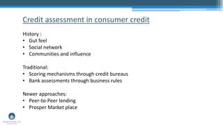
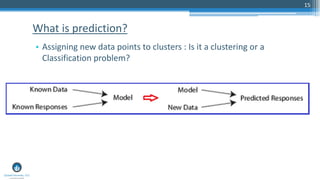
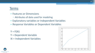
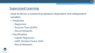
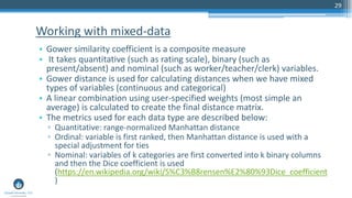
Location:
QuantUniversity Meetup
October 28th 2016
Boston MA
Machine Learning applications for Credit Risk
2016 Copyright QuantUniversity LLC.
Presented By:
Sri Krishnamurthy, CFA, CAP
www.QuantUniversity.com
sri@quantuniversity.com
2
Slides and Code will be available at:
http://www.analyticscertificate.com
- Analytics Advisory services
- Custom training programs
- Architecture assessments, advice and audits
• Founder of QuantUniversity LLC. and
www.analyticscertificate.com
• Advisory and Consultancy for Financial Analytics
• Prior Experience at MathWorks, Citigroup and
Endeca and 25+ financial services and energy
customers.
• Regular Columnist for the Wilmott Magazine
• Author of forthcoming book
“Financial Modeling: A case study approach”
published by Wiley
• Charted Financial Analyst and Certified Analytics
Professional
• Teaches Analytics in the Babson College MBA
program and at Northeastern University, Boston
Sri Krishnamurthy
Founder and CEO
4
5
Quantitative Analytics and Big Data Analytics Onboarding
• Trained more than 500 students in
Quantitative methods, Data Science
and Big Data Technologies using
MATLAB, Python and R
• Launching the Analytics Certificate
Program in September
7
Credit risk in consumer credit
Credit-scoring models and techniques assess the risk in lending to
customers.
Typical decisions:
• Grant credit/not to new applicants
• Increasing/Decreasing spending limits
• Increasing/Decreasing lending rates
• What new products can be given to existing applicants ?
Credit assessment in consumer credit
History :
• Gut feel
• Social network
• Communities and influence
Traditional:
• Scoring mechanisms through credit bureaus
• Bank assessments through business rules
Newer approaches:
• Peer-to-Peer lending
• Prosper Market place
10
• The paper finds a link between
having a high credit score and the
likelihood of both entering into a
committed relationship, and
staying in one.
Credit risk in the news
https://www.federalreserve.gov/econresdata/feds/2015/files/2
015081pap.pdf
11
12
13
14
Another methodology
15
• Assigning new data points to clusters : Is it a clustering or a
Classification problem?
What is prediction?
16
Types of algorithms
Machine
learning
Supervised
Learning
Prediction
Classification
Unsupervised
Learning
Clustering
17
• Features or Dimensions
▫ Attributes of data used for modeling
• Explanatory variables or Independent Variables
• Response Variables or Dependent Variables
Y = F(Xi)
Y = Dependent Variable
Xi = Independent Variables
Terms
18
• Numerical variables
▫ Real
 Temperature : 61.4F, 58F
▫ Integers
 Number of Bedrooms : 2,3,4
• Categorical variables
▫ Binary
 Gas-heat : Yes/No
▫ Nominal : No intrinsic ordering
 Boston, New York, Chicago
▫ Ordinal : Ordered
 Small, Medium, Large
Types of variables
19
Used to derive a relationship between dependent and independent
variables
• Prediction
▫ Regression
▫ Decision Trees (CART)
▫ Neural Networks
• Classification
▫ Logistic Regression
▫ CART, Random Forest, SVM
▫ Neural Networks
Supervised Learning
20
Data pre-
processing
Split Data into
Training and
Testing sets
Train the model
on Training data
Test the model
using Testing data
to evaluate model
performance
Methodology
21
• No distinction between independent variables and dependent
variables
• No result labels to determine “correct” results
• Goals:
▫ Data Reduction
▫ Clustering
Unsupervised Learning
22
• The goal is to find similarities in the training data and to partition
the dataset into subsets that are demarcated by these similarities.
• The clusters are not labeled but the labels are deduced through
review of the members of the clusters.
• Works well when large amounts of data available.
Clustering
23
• Partitioning Clustering
▫ Starts with K –number of clusters sought
▫ Observations randomly divided to form cohesive clusters
▫ Example : K-means
• Hierarchical Agglomerative Clustering
▫ Each observation is its own cluster
▫ Combine clusters two at a time to finally have one cluster
▫ Example: Hierarchical clustering using single linkage, Ward’s method
etc.
Types of Clustering
24
• Tries to separate samples into K groups with a goal of maximizing
between group variance and minimizing within group variance
• Requires K to be specified up front.
• Starts with K initial centroids and optimizes to minimize the criterion
or till the number of specified iterations are reached.
• Suited for larger datasets
• http://shabal.in/visuals/kmeans/3.html
K-means
25
• Goal is to derive a dendrogram starting from each record being its
own cluster
• Works well for smaller data sets
• Proximity is measured in multiple ways (more later)
Hierarchical clustering
26
How do you measure similarity between two entities ?
▫ Apples and Bananas
▫ Coke and Pepsi vs Orange juice
▫ Honda Civic vs Toyota Corolla
▫ New York and Boston
• The notion of distance
The notion of distance
27
• Euclidean distance
• Cosine distance
Distance measures
28
• Manhattan distance
(Taxi-cab distance)
• Jaccard distance
▫ Used to measure similarity or dissimilarity between binary and non-
binary variables
▫ http://people.revoledu.com/kardi/tutorial/Similarity/Jaccard.html
Other distance measures
29
• Gower similarity coefficient is a composite measure
• It takes quantitative (such as rating scale), binary (such as
present/absent) and nominal (such as worker/teacher/clerk) variables.
• Gower distance is used for calculating distances when we have mixed
types of variables (continuous and categorical)
• A linear combination using user-specified weights (most simple an
average) is calculated to create the final distance matrix.
• The metrics used for each data type are described below:
▫ Quantitative: range-normalized Manhattan distance
▫ Ordinal: variable is first ranked, then Manhattan distance is used with a
special adjustment for ties
▫ Nominal: variables of k categories are first converted into k binary columns
and then the Dice coefficient is used
(https://en.wikipedia.org/wiki/S%C3%B8rensen%E2%80%93Dice_coefficient
)
Working with mixed-data
30
• daisy
• Pam
• agnes
https://stat.ethz.ch/R-manual/R-devel/library/cluster/html/pam.html
https://en.wikibooks.org/wiki/Data_Mining_Algorithms_In_R/Clusteri
ng/CLARA
Support in R
31
32
Lending club
33
The Data
https://www.lendingclub.com/info/download-data.action
34
The Data
https://www.kaggle.com/wendykan/lending-club-loan-data
Variable description
• Calculate dissimilarity between observations.
• Select algorithm to group observations together
• Choose the best number of clusters
• Visualize clusters on reduced dimensions
Objective
• Partitioning around medoids (PAM) is used in this case.
• PAM is an iterative clustering procedure with the following steps:
▫ Step 1: Choose k random entities to become the medoids.
▫ Step 2: Assign every entity to its closest medoid (using the distance
matrix we have calculated).
▫ Step 3: For each cluster, identify the observation that would yield the
lowest average distance if it were to be re-assigned as the medoid. If
so, make this observation the new medoid.
▫ Step 4: If at least one medoid has changes, return to step 2.
Otherwise, end the algorithm.
Selecting number of clusters
• One way to visualize many variables in a lower dimensional space is
with t-distributed stochastic neighborhood embedding (t-SNE)
• This method is a dimension reduction technique that tries to
preserve local structure so as to make clusters visible in a 2D or 3D
visualization.
• https://en.wikipedia.org/wiki/T-
distributed_stochastic_neighbor_embedding
Visualization with reduced dimension
Thank you!
Members & Sponsors!
Sri Krishnamurthy, CFA, CAP
Founder and CEO
QuantUniversity LLC.
srikrishnamurthy
www.QuantUniversity.com
Contact
Information, data and drawings embodied in this presentation are strictly a property of QuantUniversity LLC. and shall not be
distributed or used in any other publication without the prior written consent of QuantUniversity LLC.
39

Credit risk meetup

  • 1.
    Location: QuantUniversity Meetup October 28th2016 Boston MA Machine Learning applications for Credit Risk 2016 Copyright QuantUniversity LLC. Presented By: Sri Krishnamurthy, CFA, CAP www.QuantUniversity.com sri@quantuniversity.com
  • 2.
    2 Slides and Codewill be available at: http://www.analyticscertificate.com
  • 3.
    - Analytics Advisoryservices - Custom training programs - Architecture assessments, advice and audits
  • 4.
    • Founder ofQuantUniversity LLC. and www.analyticscertificate.com • Advisory and Consultancy for Financial Analytics • Prior Experience at MathWorks, Citigroup and Endeca and 25+ financial services and energy customers. • Regular Columnist for the Wilmott Magazine • Author of forthcoming book “Financial Modeling: A case study approach” published by Wiley • Charted Financial Analyst and Certified Analytics Professional • Teaches Analytics in the Babson College MBA program and at Northeastern University, Boston Sri Krishnamurthy Founder and CEO 4
  • 5.
    5 Quantitative Analytics andBig Data Analytics Onboarding • Trained more than 500 students in Quantitative methods, Data Science and Big Data Technologies using MATLAB, Python and R • Launching the Analytics Certificate Program in September
  • 7.
  • 8.
    Credit risk inconsumer credit Credit-scoring models and techniques assess the risk in lending to customers. Typical decisions: • Grant credit/not to new applicants • Increasing/Decreasing spending limits • Increasing/Decreasing lending rates • What new products can be given to existing applicants ?
  • 9.
    Credit assessment inconsumer credit History : • Gut feel • Social network • Communities and influence Traditional: • Scoring mechanisms through credit bureaus • Bank assessments through business rules Newer approaches: • Peer-to-Peer lending • Prosper Market place
  • 10.
    10 • The paperfinds a link between having a high credit score and the likelihood of both entering into a committed relationship, and staying in one. Credit risk in the news https://www.federalreserve.gov/econresdata/feds/2015/files/2 015081pap.pdf
  • 11.
  • 12.
  • 13.
  • 14.
  • 15.
    15 • Assigning newdata points to clusters : Is it a clustering or a Classification problem? What is prediction?
  • 16.
  • 17.
    17 • Features orDimensions ▫ Attributes of data used for modeling • Explanatory variables or Independent Variables • Response Variables or Dependent Variables Y = F(Xi) Y = Dependent Variable Xi = Independent Variables Terms
  • 18.
    18 • Numerical variables ▫Real  Temperature : 61.4F, 58F ▫ Integers  Number of Bedrooms : 2,3,4 • Categorical variables ▫ Binary  Gas-heat : Yes/No ▫ Nominal : No intrinsic ordering  Boston, New York, Chicago ▫ Ordinal : Ordered  Small, Medium, Large Types of variables
  • 19.
    19 Used to derivea relationship between dependent and independent variables • Prediction ▫ Regression ▫ Decision Trees (CART) ▫ Neural Networks • Classification ▫ Logistic Regression ▫ CART, Random Forest, SVM ▫ Neural Networks Supervised Learning
  • 20.
    20 Data pre- processing Split Datainto Training and Testing sets Train the model on Training data Test the model using Testing data to evaluate model performance Methodology
  • 21.
    21 • No distinctionbetween independent variables and dependent variables • No result labels to determine “correct” results • Goals: ▫ Data Reduction ▫ Clustering Unsupervised Learning
  • 22.
    22 • The goalis to find similarities in the training data and to partition the dataset into subsets that are demarcated by these similarities. • The clusters are not labeled but the labels are deduced through review of the members of the clusters. • Works well when large amounts of data available. Clustering
  • 23.
    23 • Partitioning Clustering ▫Starts with K –number of clusters sought ▫ Observations randomly divided to form cohesive clusters ▫ Example : K-means • Hierarchical Agglomerative Clustering ▫ Each observation is its own cluster ▫ Combine clusters two at a time to finally have one cluster ▫ Example: Hierarchical clustering using single linkage, Ward’s method etc. Types of Clustering
  • 24.
    24 • Tries toseparate samples into K groups with a goal of maximizing between group variance and minimizing within group variance • Requires K to be specified up front. • Starts with K initial centroids and optimizes to minimize the criterion or till the number of specified iterations are reached. • Suited for larger datasets • http://shabal.in/visuals/kmeans/3.html K-means
  • 25.
    25 • Goal isto derive a dendrogram starting from each record being its own cluster • Works well for smaller data sets • Proximity is measured in multiple ways (more later) Hierarchical clustering
  • 26.
    26 How do youmeasure similarity between two entities ? ▫ Apples and Bananas ▫ Coke and Pepsi vs Orange juice ▫ Honda Civic vs Toyota Corolla ▫ New York and Boston • The notion of distance The notion of distance
  • 27.
    27 • Euclidean distance •Cosine distance Distance measures
  • 28.
    28 • Manhattan distance (Taxi-cabdistance) • Jaccard distance ▫ Used to measure similarity or dissimilarity between binary and non- binary variables ▫ http://people.revoledu.com/kardi/tutorial/Similarity/Jaccard.html Other distance measures
  • 29.
    29 • Gower similaritycoefficient is a composite measure • It takes quantitative (such as rating scale), binary (such as present/absent) and nominal (such as worker/teacher/clerk) variables. • Gower distance is used for calculating distances when we have mixed types of variables (continuous and categorical) • A linear combination using user-specified weights (most simple an average) is calculated to create the final distance matrix. • The metrics used for each data type are described below: ▫ Quantitative: range-normalized Manhattan distance ▫ Ordinal: variable is first ranked, then Manhattan distance is used with a special adjustment for ties ▫ Nominal: variables of k categories are first converted into k binary columns and then the Dice coefficient is used (https://en.wikipedia.org/wiki/S%C3%B8rensen%E2%80%93Dice_coefficient ) Working with mixed-data
  • 30.
    30 • daisy • Pam •agnes https://stat.ethz.ch/R-manual/R-devel/library/cluster/html/pam.html https://en.wikibooks.org/wiki/Data_Mining_Algorithms_In_R/Clusteri ng/CLARA Support in R
  • 31.
  • 32.
  • 33.
  • 34.
  • 35.
  • 36.
    • Calculate dissimilaritybetween observations. • Select algorithm to group observations together • Choose the best number of clusters • Visualize clusters on reduced dimensions Objective
  • 37.
    • Partitioning aroundmedoids (PAM) is used in this case. • PAM is an iterative clustering procedure with the following steps: ▫ Step 1: Choose k random entities to become the medoids. ▫ Step 2: Assign every entity to its closest medoid (using the distance matrix we have calculated). ▫ Step 3: For each cluster, identify the observation that would yield the lowest average distance if it were to be re-assigned as the medoid. If so, make this observation the new medoid. ▫ Step 4: If at least one medoid has changes, return to step 2. Otherwise, end the algorithm. Selecting number of clusters
  • 38.
    • One wayto visualize many variables in a lower dimensional space is with t-distributed stochastic neighborhood embedding (t-SNE) • This method is a dimension reduction technique that tries to preserve local structure so as to make clusters visible in a 2D or 3D visualization. • https://en.wikipedia.org/wiki/T- distributed_stochastic_neighbor_embedding Visualization with reduced dimension
  • 39.
    Thank you! Members &Sponsors! Sri Krishnamurthy, CFA, CAP Founder and CEO QuantUniversity LLC. srikrishnamurthy www.QuantUniversity.com Contact Information, data and drawings embodied in this presentation are strictly a property of QuantUniversity LLC. and shall not be distributed or used in any other publication without the prior written consent of QuantUniversity LLC. 39