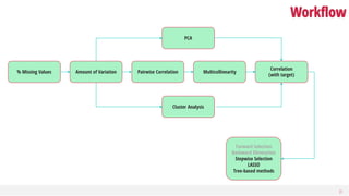
This document discusses dimensionality reduction, a vital process in machine learning that involves selecting a subset of features for model construction. It outlines various techniques such as principal component analysis, cluster analysis, and selection methods to manage the challenges of high-dimensional data and the curse of dimensionality. The guide emphasizes the importance of reducing redundancy and irrelevant features to enhance predictive power and model efficiency.

1. Vishal Patel
October 8, 2016
1
A Practical Guide to Dimensionality Reduction

2. 2
WhoAmI
 Vishal Patel
 Data Science Consultant
 Founder of DERIVE, LLC
 Fully Automated Advanced Analytics products
 Have been mining data for about a decade and a half
 MS in Computer Science, and MS in Decision Sciences (emphasis on Statistics)
 Richmond, VA
w w w . d e r i v e . i o

3. Agenda
Dimensionality Reduction
What When Why How Q&A
5-7 minutes 25 minutes 5-10 minutes

4. 4
What
 Dimensionality Reduction: The process of selecting a subset of features for use in model construction
 Pre-processing of data in machine learning
 Can be useful for both supervised and unsupervised learning problems, but we will focus on the former
“Art is the elimination of the unnecessary.“
Pablo Picasso

5. 5
When (Process Flow)
Business Problem
Data Collection Data Discovery Vectorization Data Preparation
ModelingEvaluationDeploymentTracking
Combine data, create features, tabular format Impute, transform, feature reduction
Machine Learning, model trainingModel validation and selectionModel decay tracking
Model refinement
Productionalize
Continuous Feedback Loop

6. 6
Dataset
https://www.kaggle.com/c/springleaf-marketing-response/data
Train Test
1,933 1,933 features
145,231 145,232 records
Anonymized features  Predict which customers will respond to a DM offer
Challenge: To construct new meta-variables and employ feature-selection methods to
approach this dauntingly wide dataset.

7. 7
Why Not This
The kitchen sink approach

8. 8
Because…
 True dimensionality <<< Observed dimensionality
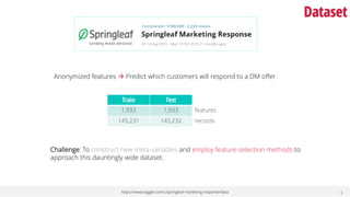
 The abundance of redundant and irrelevant features
 Curse of dimensionality
 With a fixed number of training samples, the predictive power reduces as the dimensionality increases.
[Hughes phenomenon]
 With 𝑑 binary variables, the number of possible combinations is 𝑂(2 𝑑
).
 Value of Analytics
 Descriptive  Diagnostic  Predictive  Prescriptive
 Law of Parsimony [Occam’s Razor]
 Other things being equal, simpler explanations are generally better than complex ones.
 Overfitting
 Execution time (Algorithm and data)
Hindsight Insight Foresight

9. 9
How
1. Percent missing values
2. Amount of variation
3. Pairwise correlation
4. Multicolinearity
5. Principal Component Analysis (PCA)
6. Cluster analysis
7. Correlation (with the target)
8. Forward selection
9. Backward elimination
10. Stepwise selection
11. LASSO
12. Tree-based selection
Information
Redundancy
Predictive Power
Greedy Selection
Embedded
Dimensionality
Reduction
Techniques

10. 10
1. Percent Missing Values
 Drop variables that have a very high % of missing values
 # of records with missing values / # of total records
 Create binary indicators to denote missing (or non-missing) values
 Review or visualize variables with high % of missing values

11. 11
1. Percent Missing Values
> 95% DISCARD
50% to 95%
NO IMPUTATION
< 50%
IMPUTATION
<= 95%
MISSING
VALUE
INDICATORS
% Missing

12. 12
2. Amount of Variation
 Drop or review variables that have a very low variation
 𝑽𝑨𝑹 𝒙 = 𝝈 𝟐
=
𝟏
𝒏
σ𝒊=𝟏
𝒏
(𝒙𝒊 − 𝝁) 𝟐
 Either standardize all variables, or use standard deviation 𝜎 to account
for variables with difference scales
 Drop variables with zero variation (unary)

13. 13
2. Amount of Variation
Drop 39 fields
with zero variation
Standard Deviation
(less than one)

14. 14
3. Pairwise Correlations
 Many variables are often correlated with each other, and hence are redundant.
 If two variables are highly correlated, keeping only one will help reduce dimensionality without
much loss of information.
 Which variable to keep? The one that has a higher correlation coefficient with the target.

15. 15
3. Pairwise Correlations
𝑥1 𝑥2 𝑥3 𝑥4
𝑥1 1.00 0.15 0.85 0.01
𝑥2 1.00 0.45 0.60
𝑥3 1.00 0.17
𝑥4 1.00
𝑦
𝑥1 0.67
𝑥2 0.82
𝑥3 0.58
𝑥4 0.25
Keep 𝑥1, Discard 𝑥3
Correlation tolerance ≈ 0.65
1. Identify pairs of highly correlated variables 2. Discard variable with weaker correlation with the target

16. 16
3. Pairwise Correlations

17. 17
4. Multicolinearity
 When two or more variables are highly correlated with each other.
 Dropping one or more variables should help reduce dimensionality without a substantial loss of
information.
 Which variable(s) to drop? Use Condition Index.
𝑥1 𝑥2 𝑥3 𝑥4
𝑥1 1.00 0.15 0.85 0.01
𝑥2 1.00 0.45 0.60
𝑥3 1.00 0.17
𝑥4 1.00
Condition
Index
𝑥1 𝑥2 𝑥3 𝑥4
𝑢1 = 1.0 0.01 0.05 0.00 0.16
𝑢2 = 16.5 0.03 0.12 0.01 0.19
𝑢3 = 28.7 0.05 0.02 0.13 0.25
𝑢4 = 97.1 0.93 0.91 0.98 0.11 Discard 𝑥3, Iterate
Condition Index tolerance ≈ 0.30

18. 18
4. Multicolinearity

19. 19
4. Multicolinearity

20. 20
5. Principal Component Analysis (PCA)
 Dimensionality reduction technique which emphasizes variation.
 Eliminates multicollinearity – but explicability is compromised.
 Uses orthogonal transformation
 When to use:
 Excessive multicollinearity
 Explanation of the predictors is not important.
 A slight overhead in implementation is okay.

21. 21
5. PCA
 Scree plot: Elbow in the curve
 % Variance Explained
 Eigenvalue >= 1
 Number of components retained
% Variance Explained Cumulative
% Variance Explained

22. 22
5. PCA

23. 23
6. Cluster Analysis
 Dimensionality reduction technique which emphasizes correlation/similarity.
 Identify groups of variables that are as correlated as possible among themselves
and as uncorrelated as possible with variables in other clusters.
 Reduces multicollinearity – and explicability is not (always) compromised.
 When to use:
 Excessive multicollinearity.
 Explanation of the predictors is important.
𝑥1
𝑥4
𝑥2
𝑥3
Two clusters

24. 24
6. Cluster Analysis
 This returns a pooled value for each cluster (i.e., the centroids), which can then be used to
build a supervised learning model.
 In SAS, using PROC VARCLUS you can choose one variable from each cluster that is the
most representative of that cluster.
 Use 1 − 𝑅2 ratio to select a variable from each cluster.
http://scikit-learn.org/stable/modules/generated/sklearn.cluster.FeatureAgglomeration.html#sklearn.cluster.FeatureAgglomeration

25. 25
7. Correlation with the Target
 Drop variables that have a very low correlation with the target.
 If a variable has a very low correction with the target, it’s not going to useful
for the model (prediction).

26. 26
7. Correlation with the Target
 Elbow in the curve
 Absolute correlation
 Number of variables retained

27. 27
8-10. Forward/Backward/Stepwise Selection
 Forward Selection
1. Identify the best variable (e.g., based on model accuracy)
2. Add the next best variable into the model
3. And so on until some predefined criteria is satisfied.
 Backward Elimination
1. Start with all variables included in the model.
2. Drop the least useful variable (e.g., based on the smallest drop in model accuracy)
3. And so on until some predefined criteria is satisfied.
 Stepwise Selection
 Similar to forward selection process, but a variable can also be dropped if it’s
deemed as not useful any more after a certain number of steps.

28. 28
10. Stepwise Selection

29. 29
11. LASSO
 Least Absolute Shrinkage and Selection Operator
 Two birds, one stone: Variable Selection + Regularization

30. 30
12. Tree-based
 Forests of trees to evaluate the importance of features
 Fit a number of randomized decision trees on various sub-samples of the dataset
and use averaging to rank order features

31. 31
Workflow
% Missing Values Amount of Variation Pairwise Correlation Multicollinearity
Correlation
(with target)
Cluster Analysis
PCA
Forward Selection
Backward Elimination
Stepwise Selection
LASSO
Tree-based methods

32. 32
Comparisons
AUC

33. 33
The Kitchen Sink Approach
AUC

34. 34
Dimensionality Reduction
All you can eat Eat healthy

35. THANK YOU!
QUESTIONS?
vishal@derive.io
www.linkedIn.com/in/VishalJP