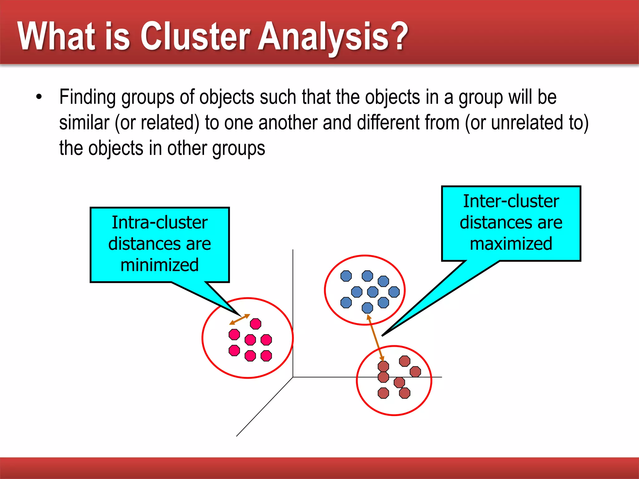
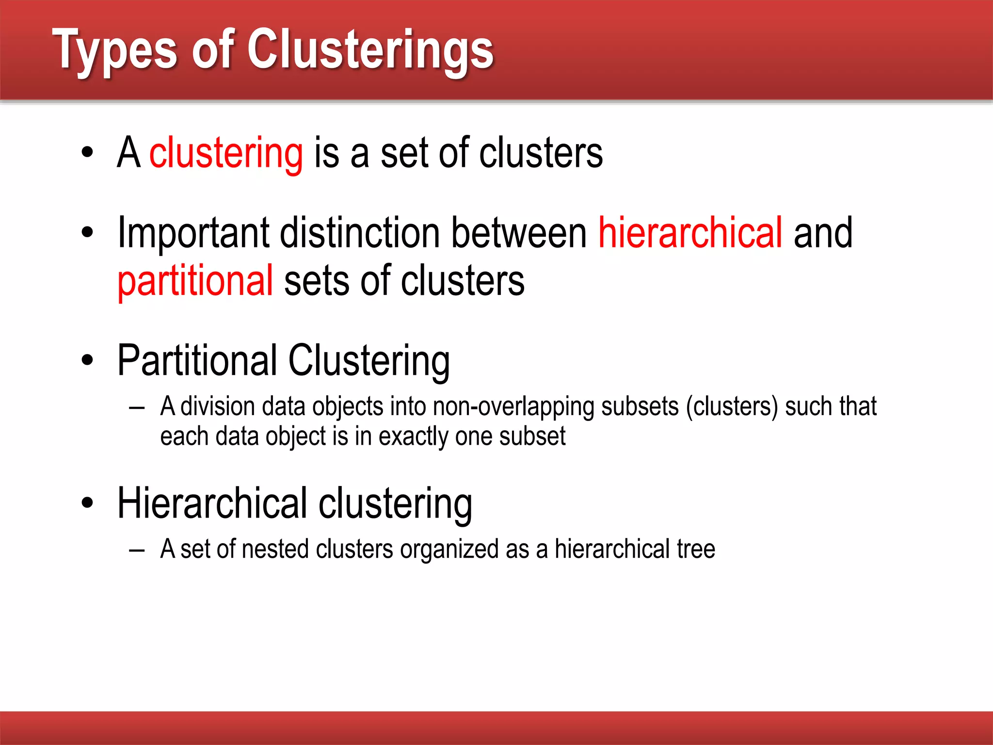
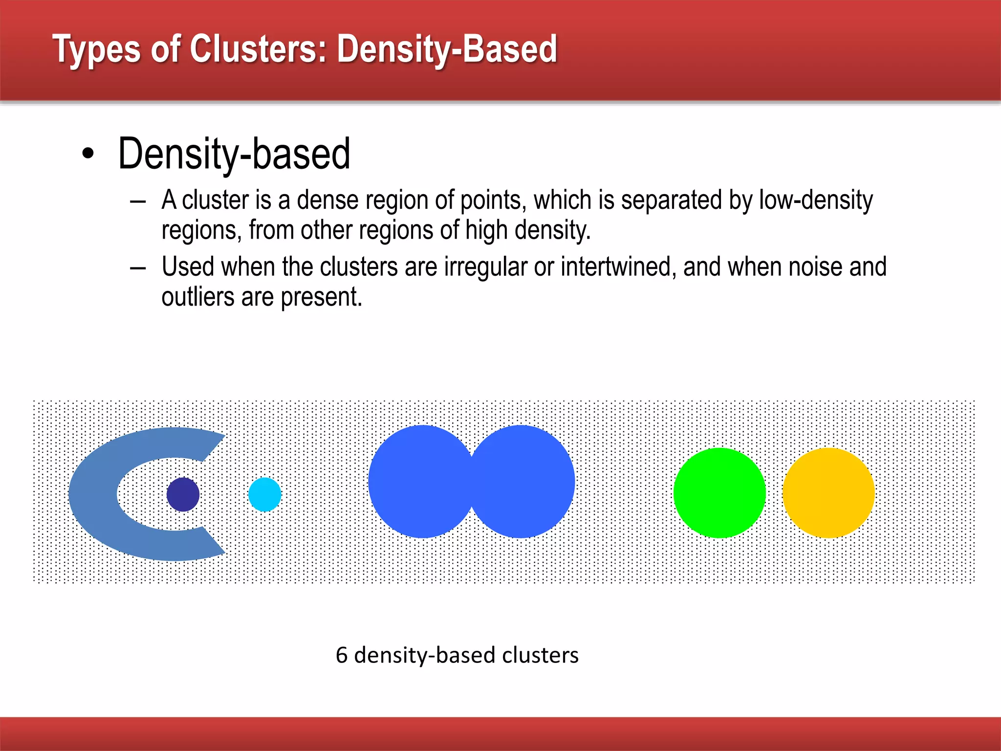
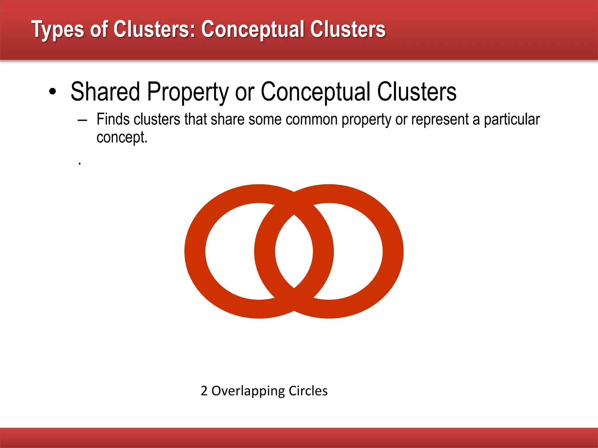
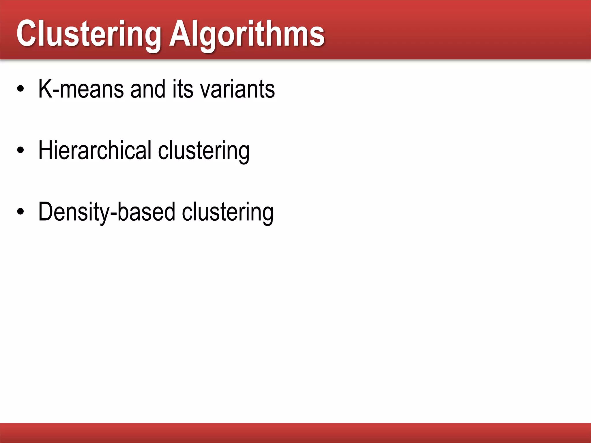
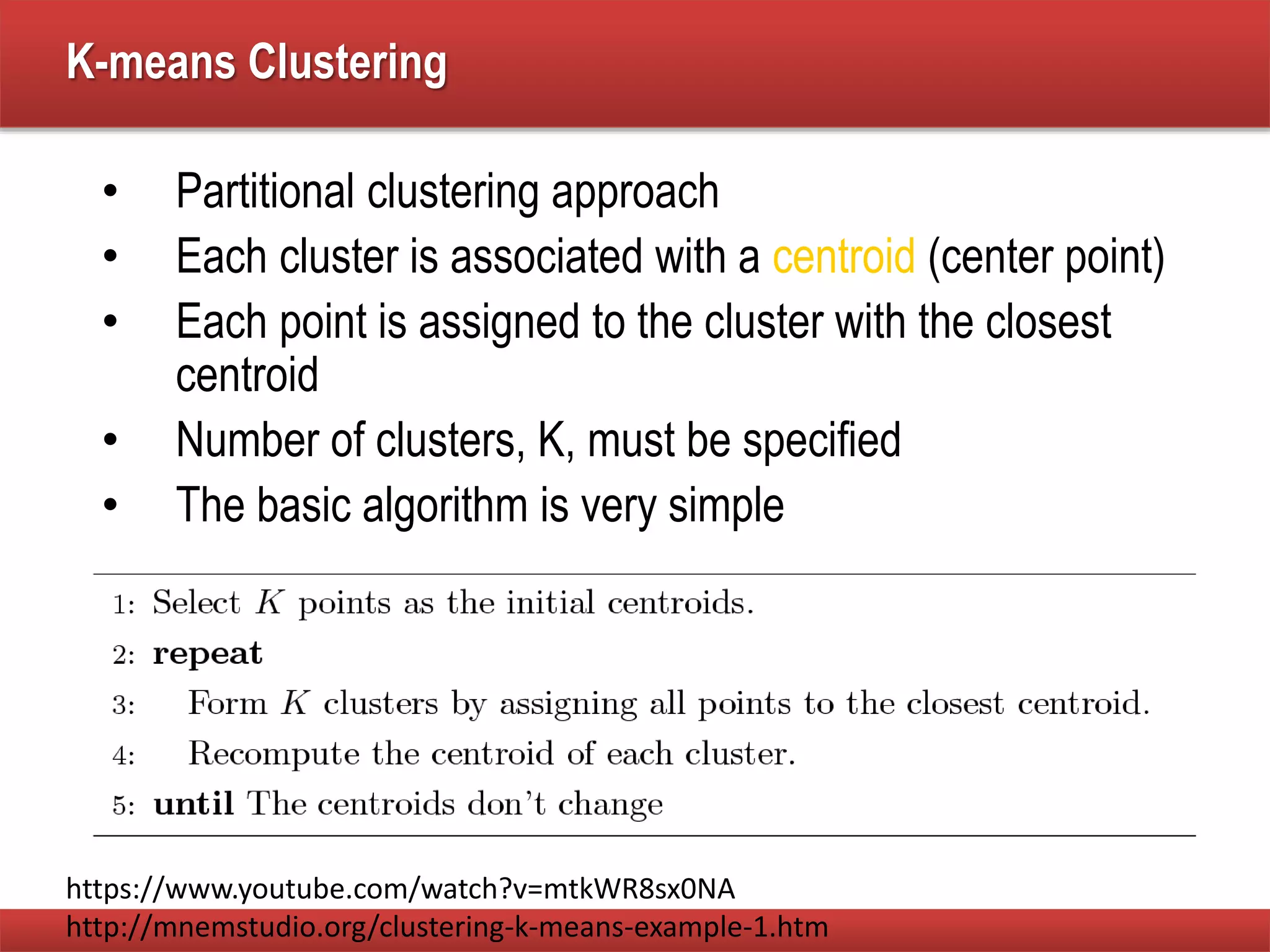
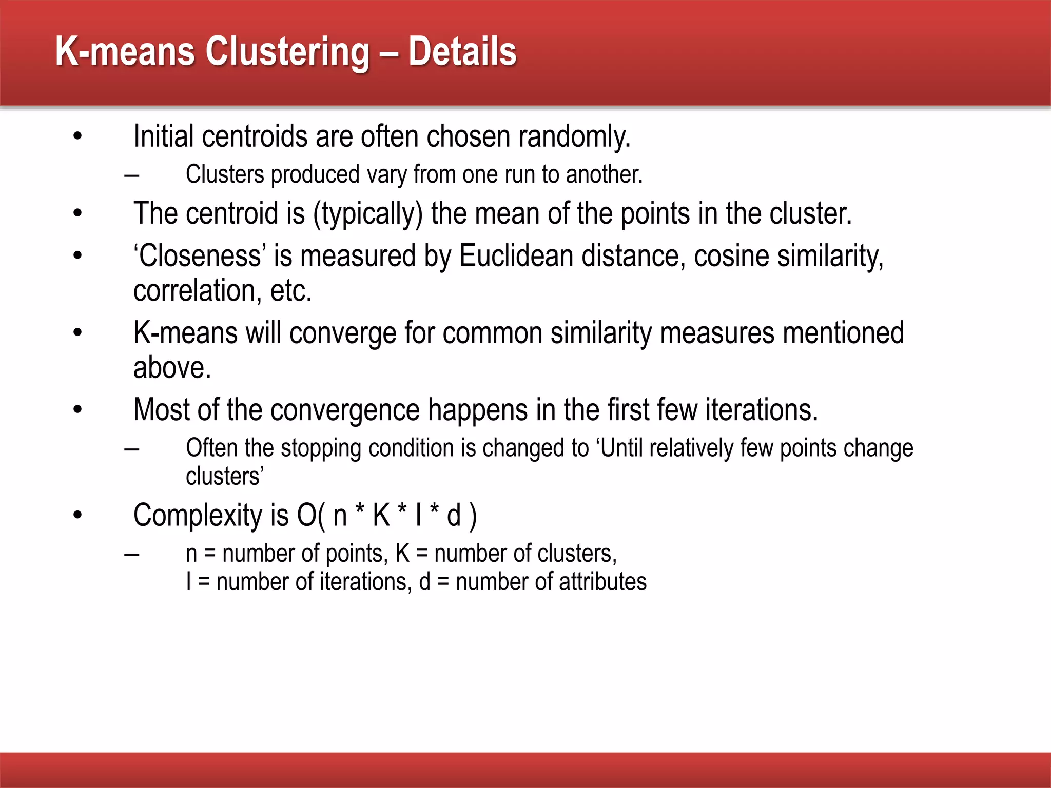
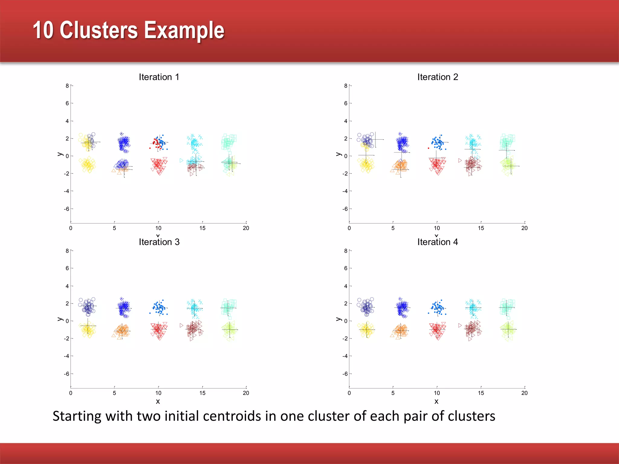
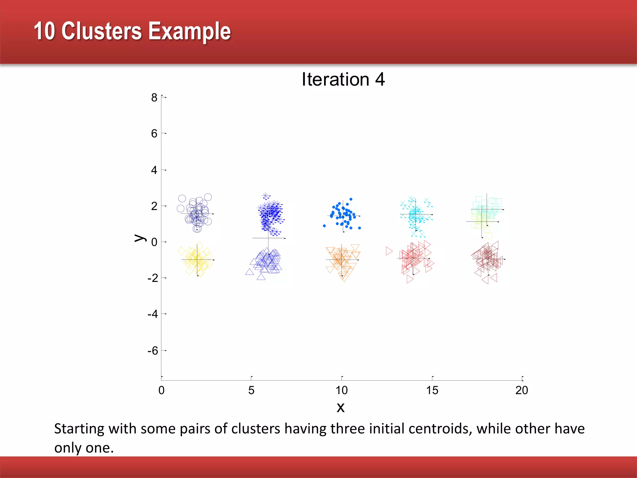
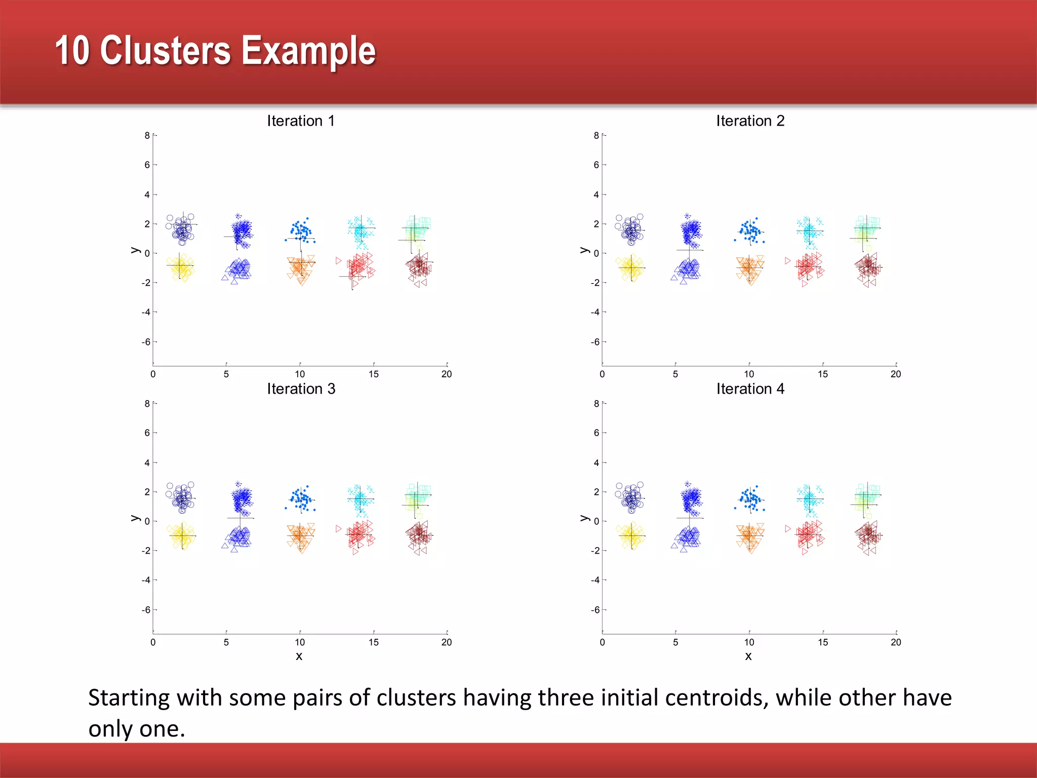
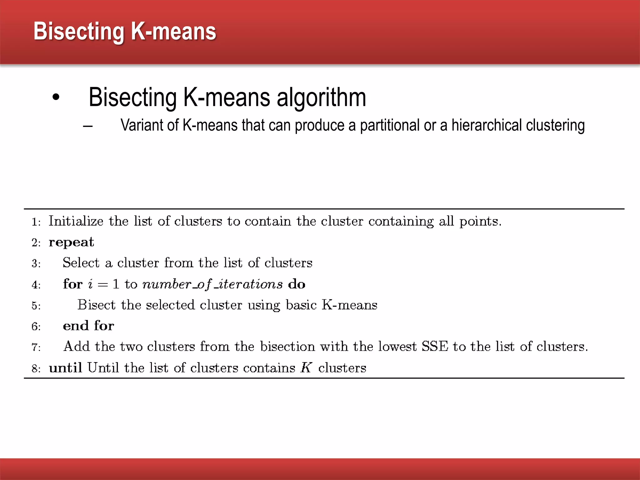
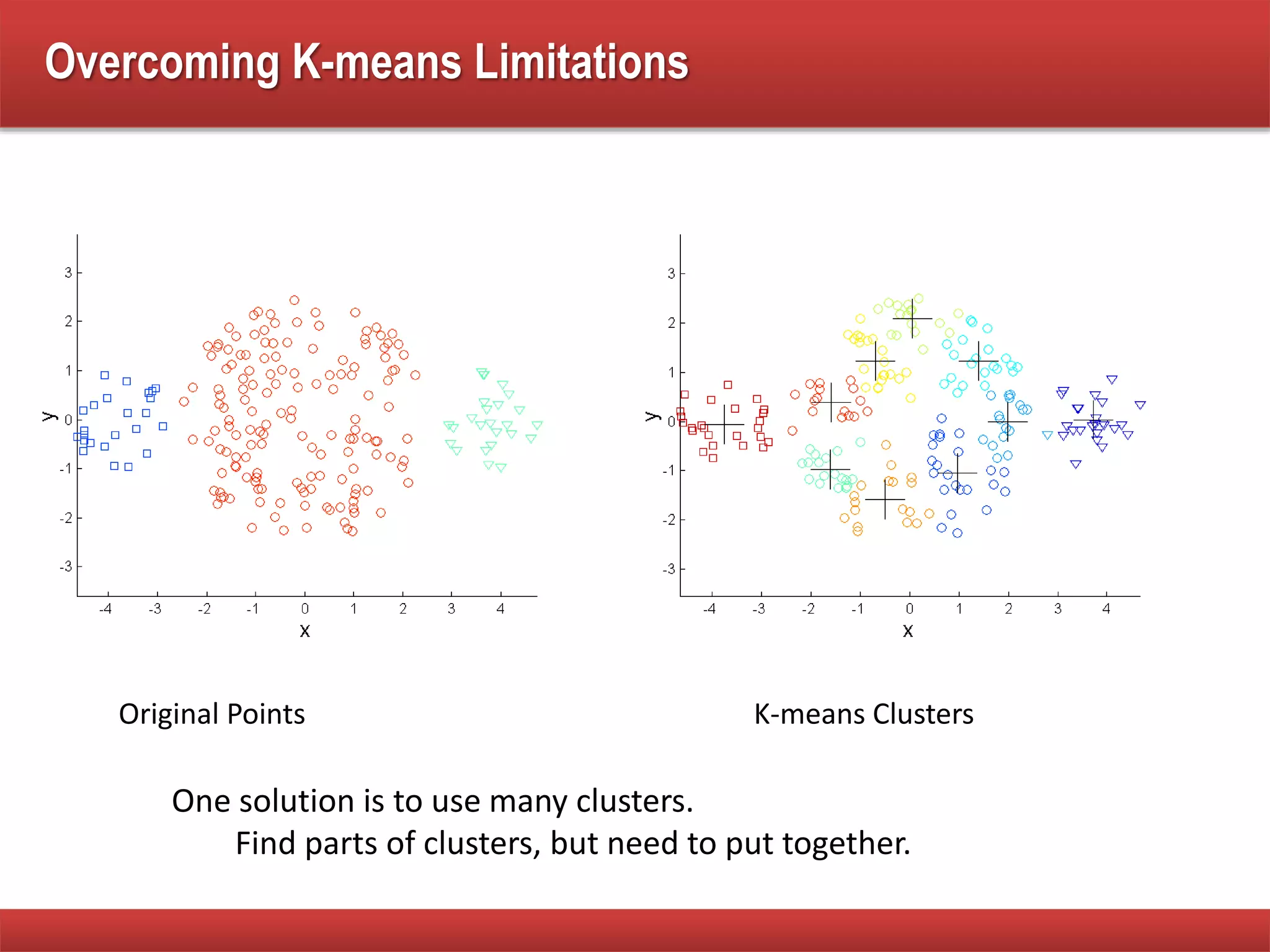
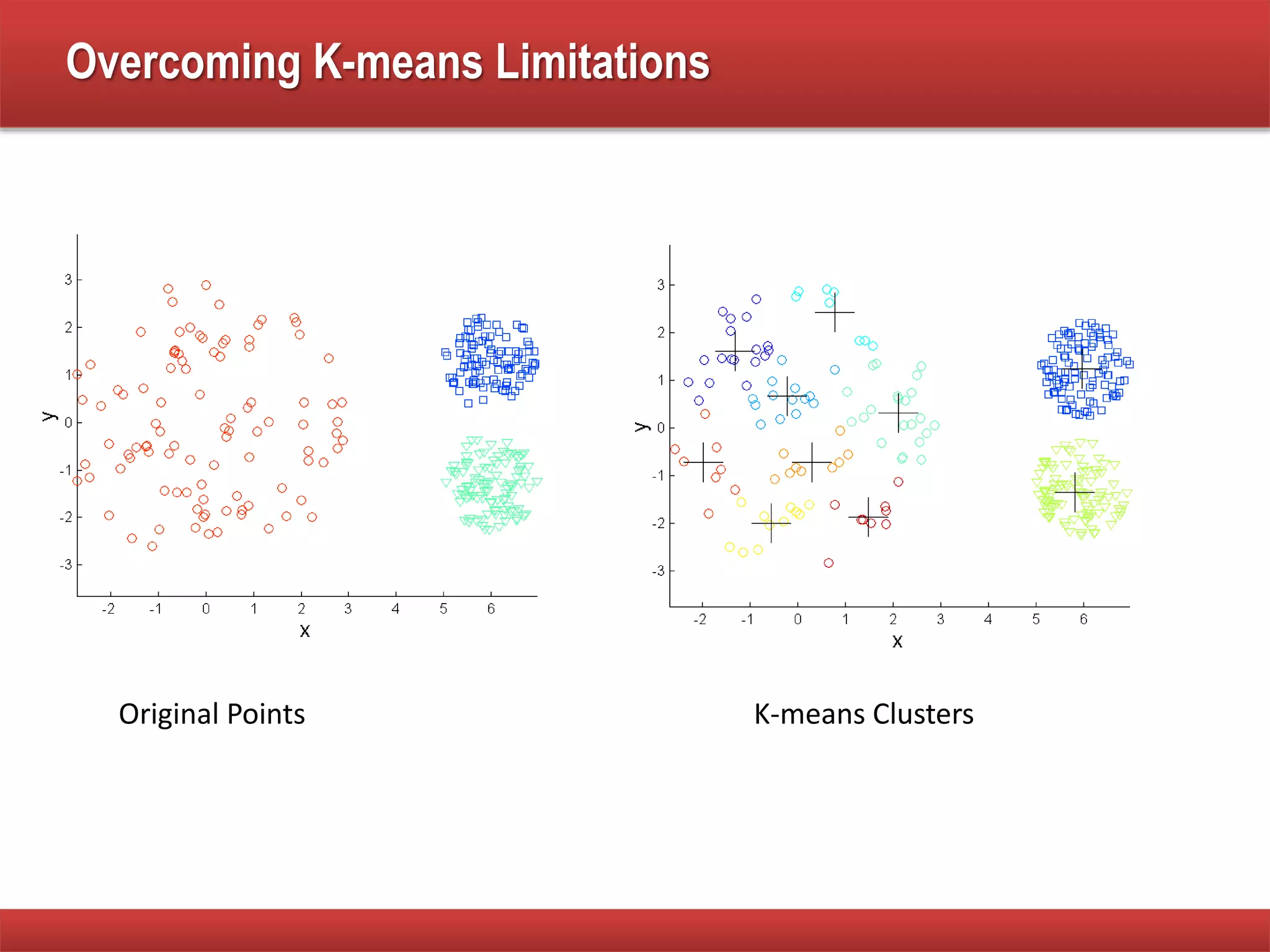
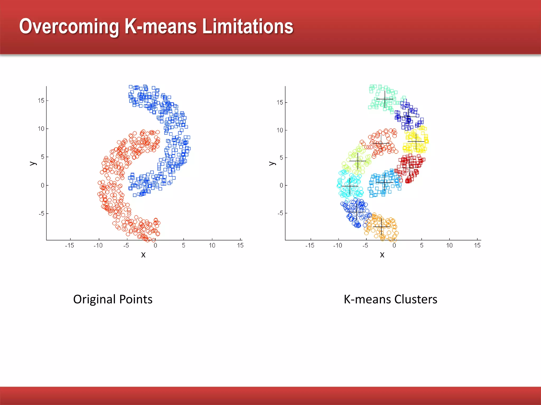
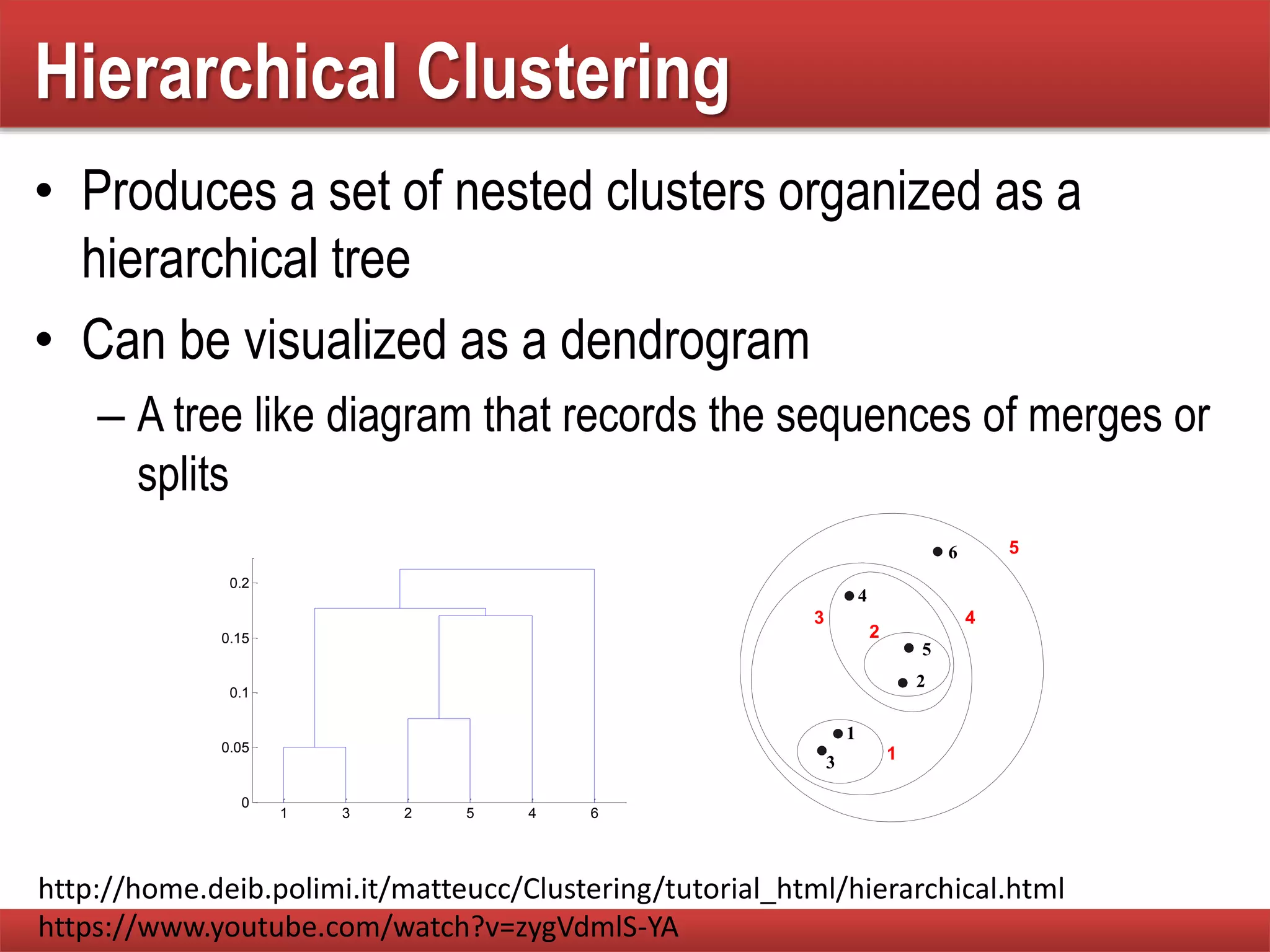
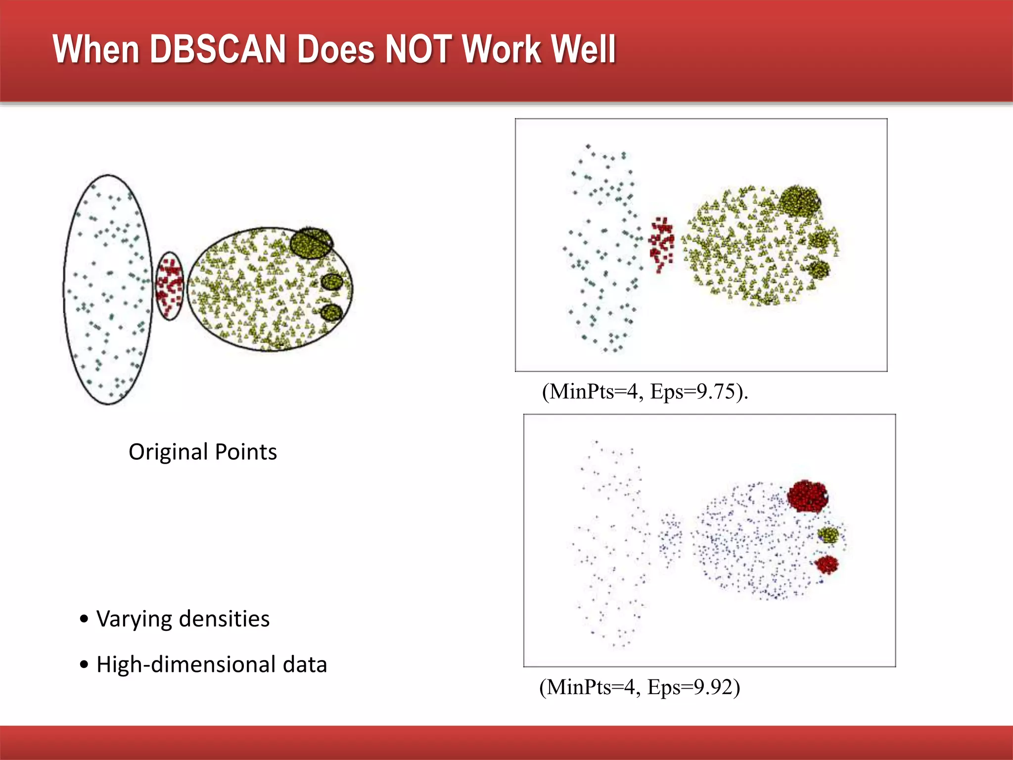
This slide is all about the Data mining techniques.This slide is all about the Data mining techniques.This slide is all about the Data mining techniques.This slide is all about the Data mining techniques;This slide is all about the Data mining techniques;This slide is all about the Data mining techniques.This slide is all about the Data mining techniques.This slide is all about the Data mining techniques

1. Data Mining
Lecture – 05

2. What is Cluster Analysis?
• Finding groups of objects such that the objects in a group will be
similar (or related) to one another and different from (or unrelated to)
the objects in other groups
Inter-cluster
distances are
maximized
Intra-cluster
distances are
minimized

3. Clustering for Understanding
• Classes, or conceptually meaningful groups of objects that
share common characteristics, play an important role in how
people analyze and describe the world.
• Indeed, human beings are skilled at dividing objects into groups
(clustering) and assigning particular objects to these groups
(classification).
• For example, even relatively young children can quickly label
the objects in a photograph as buildings, vehicles, people,
animals, plants, etc.
• In the context of understanding data, clusters are potential
classes and cluster analysis is the study of techniques for
automatically finding classes.

4. Clustering for Understanding - Example
• Biology
– Biologist have applied clustering to analyze the large amounts of
genetic information that are now available. For example, clustering has
been used to find groups of genes that have similar functions.
• Information Retrieval
– Clustering can be used to group search results (from a search engine)
into a smaller number of clusters, each of which captures a particular
aspect of the query. For instance, a query "movie" might return Web
pages groups into categories such as reviews, trailers, stars, and
theaters.

5. Clustering for Understanding - Example
• Climate
– Cluster analysis has been applied to find patterns in the atmospheric
pressure of polar regions and areas of the ocean that have significant
impact of land climate.
• Psychology and Medicine
– An illness or condition frequently has a number of variations, and
cluster analysis can be used to identify these different subcategories.
For example, clustering has been used to identify different types of
depression. Cluster analysis can also be used to detect patterns in the
spatial or temporal distribution of a disease.

6. Clustering for Understanding - Example
• Business
– Businesses collect large amounts of information on current and
potential customers. Clustering can be used to segment customers into
a small number of groups for additional analysis and marketing
activities.

7. Clustering for Utility
• Some clustering techniques characterize each cluster in terms
of a cluster prototype; i.e., a data object that is representative of
the other objects in the cluster. These cluster prototypes can be
used as the basis for a number of data analysis or data
processing techniques.
• Therefore, cluster analysis is the study of techniques for finding
the most representative cluster prototypes.

8. Clustering for Utility - Example
• Summarization
– Many data analysis techniques, such as regression or PCA, have a
time or space complexity of O(m2) or higher (where m is the number of
objects), and thus, are not practical for large data sets. However,
instead of applying the algorithm to the entire data set, it can be
applied to a reduced data set consisting only of cluster prototypes.
• Compression
– Cluster prototypes can also be used for data compression. In
particular, a table is created that consists of the prototypes for each
cluster. This type of compression is known as vector quantization and
is often applied to image, sound, and video data, where (1) many of the
data objects are highly similar to one another, (2) some loss of
information is acceptable, and (3) a substantial reduction in the data
size is desired.

9. Clustering for Utility - Example
• Efficiently Finding Nearest Neighbors
– Finding nearest neighbors can require computing the pairwise distance
between all points. Often clusters and their cluster prototypes can be
found much more efficiently. If objects are relatively close to the
prototype of their cluster, then we can use the prototypes to reduce the
number of distance computations that are necessary to find the nearest
neighbors of an object. Intuitively, if two cluster prototypes are far
apart, then the objects in the corresponding clusters cannot be nearest
neighbors of each other. Consequently, to find an object's nearest
neighbors it is only necessary to compute the distance to objects in
nearby clusters, where the nearness of two clusters is measured by the
distance between their prototypes.

10. What is not Cluster Analysis?
• Supervised classification
– Have class label information
• Simple segmentation
– Dividing students into different registration groups alphabetically, by last
name
• Results of a query
– Groupings are a result of an external specification
• Graph partitioning
– Some mutual relevance and synergy, but areas are not identical

11. Notion of a Cluster can be Ambiguous
How many clusters?
Four ClustersTwo Clusters
Six Clusters

12. Types of Clusterings
• A clustering is a set of clusters
• Important distinction between hierarchical and
partitional sets of clusters
• Partitional Clustering
– A division data objects into non-overlapping subsets (clusters) such that
each data object is in exactly one subset
• Hierarchical clustering
– A set of nested clusters organized as a hierarchical tree

13. Partitional Clustering
Original Points A Partitional Clustering

14. Hierarchical Clustering
p4
p1
p3
p2
p4
p1
p3
p2
p4p1 p2 p3
p4p1 p2 p3
Traditional Hierarchical Clustering
Non-traditional Hierarchical
Clustering
Non-traditional Dendrogram
Traditional Dendrogram

15. Other Distinctions Between Sets of Clusters
• Exclusive versus non-exclusive
– Exclusive: assign each object to a single cluster
– Non-exclusive clusterings, points may belong to multiple clusters.
– Can represent multiple classes or ‘border’ points (e.g. Student as well as
Employee of a university at the same time)
• Fuzzy versus non-fuzzy
– In fuzzy clustering, a point belongs to every cluster with some weight
between 0 and 1
– Weights must sum to 1
– Probabilistic clustering has similar characteristics
• Partial versus complete
– In some cases, we only want to cluster some of the data
• Heterogeneous versus homogeneous
– Cluster of widely different sizes, shapes, and densities

16. Types of Clusters
• Well-separated clusters
• Center-based clusters
• Contiguous clusters
• Density-based clusters
• Property or Conceptual
• Described by an Objective Function

17. Types of Clusters: Well-Separated
• Well-Separated Clusters:
– A cluster is a set of points such that any point in a cluster is closer (or more
similar) to every other point in the cluster than to any point not in the cluster.
3 well-separated clusters

18. Types of Clusters: Center-Based
• Center-based
– A cluster is a set of objects such that an object in a cluster is closer (more
similar) to the “center” of a cluster, than to the center of any other cluster
– The center of a cluster is often a centroid, the average of all the points in the
cluster, or a medoid, the most “representative” point of a cluster
4 center-based clusters

19. Types of Clusters: Contiguity-Based
• Contiguous Cluster (Nearest neighbor or
Transitive)
– A cluster is a set of points such that a point in a cluster is closer (or more
similar) to one or more other points in the cluster than to any point not in the
cluster.
8 contiguous clusters

20. Types of Clusters: Density-Based
• Density-based
– A cluster is a dense region of points, which is separated by low-density
regions, from other regions of high density.
– Used when the clusters are irregular or intertwined, and when noise and
outliers are present.
6 density-based clusters

21. Types of Clusters: Conceptual Clusters
• Shared Property or Conceptual Clusters
– Finds clusters that share some common property or represent a particular
concept.
.
2 Overlapping Circles

22. Clustering Algorithms
• K-means and its variants
• Hierarchical clustering
• Density-based clustering

23. K-means Clustering
• Partitional clustering approach
• Each cluster is associated with a centroid (center point)
• Each point is assigned to the cluster with the closest
centroid
• Number of clusters, K, must be specified
• The basic algorithm is very simple
https://www.youtube.com/watch?v=mtkWR8sx0NA
http://mnemstudio.org/clustering-k-means-example-1.htm

24. K-means Clustering – Details
• Initial centroids are often chosen randomly.
– Clusters produced vary from one run to another.
• The centroid is (typically) the mean of the points in the cluster.
• ‘Closeness’ is measured by Euclidean distance, cosine similarity,
correlation, etc.
• K-means will converge for common similarity measures mentioned
above.
• Most of the convergence happens in the first few iterations.
– Often the stopping condition is changed to ‘Until relatively few points change
clusters’
• Complexity is O( n * K * I * d )
– n = number of points, K = number of clusters,
I = number of iterations, d = number of attributes

25. Two different K-means Clusterings
-2 -1.5 -1 -0.5 0 0.5 1 1.5 2
0
0.5
1
1.5
2
2.5
3
x
y
-2 -1.5 -1 -0.5 0 0.5 1 1.5 2
0
0.5
1
1.5
2
2.5
3
x
y
Sub-optimal Clustering
-2 -1.5 -1 -0.5 0 0.5 1 1.5 2
0
0.5
1
1.5
2
2.5
3
x
y
Optimal Clustering
Original Points

26. Importance of Choosing Initial Centroids
-2 -1.5 -1 -0.5 0 0.5 1 1.5 2
0
0.5
1
1.5
2
2.5
3
x
y
Iteration 1
-2 -1.5 -1 -0.5 0 0.5 1 1.5 2
0
0.5
1
1.5
2
2.5
3
x
y
Iteration 2
-2 -1.5 -1 -0.5 0 0.5 1 1.5 2
0
0.5
1
1.5
2
2.5
3
x
y
Iteration 3
-2 -1.5 -1 -0.5 0 0.5 1 1.5 2
0
0.5
1
1.5
2
2.5
3
x
y
Iteration 4
-2 -1.5 -1 -0.5 0 0.5 1 1.5 2
0
0.5
1
1.5
2
2.5
3
x
y
Iteration 5
-2 -1.5 -1 -0.5 0 0.5 1 1.5 2
0
0.5
1
1.5
2
2.5
3
x
y
Iteration 6

27. Importance of Choosing Initial Centroids
-2 -1.5 -1 -0.5 0 0.5 1 1.5 2
0
0.5
1
1.5
2
2.5
3
x
y
Iteration 1
-2 -1.5 -1 -0.5 0 0.5 1 1.5 2
0
0.5
1
1.5
2
2.5
3
x
y
Iteration 2
-2 -1.5 -1 -0.5 0 0.5 1 1.5 2
0
0.5
1
1.5
2
2.5
3
x
y
Iteration 3
-2 -1.5 -1 -0.5 0 0.5 1 1.5 2
0
0.5
1
1.5
2
2.5
3
x
y
Iteration 4
-2 -1.5 -1 -0.5 0 0.5 1 1.5 2
0
0.5
1
1.5
2
2.5
3
x
y
Iteration 5
-2 -1.5 -1 -0.5 0 0.5 1 1.5 2
0
0.5
1
1.5
2
2.5
3
x
y
Iteration 6

28. Importance of Choosing Initial Centroids …
-2 -1.5 -1 -0.5 0 0.5 1 1.5 2
0
0.5
1
1.5
2
2.5
3
x
y
Iteration 1
-2 -1.5 -1 -0.5 0 0.5 1 1.5 2
0
0.5
1
1.5
2
2.5
3
x
y
Iteration 2
-2 -1.5 -1 -0.5 0 0.5 1 1.5 2
0
0.5
1
1.5
2
2.5
3
x
y
Iteration 3
-2 -1.5 -1 -0.5 0 0.5 1 1.5 2
0
0.5
1
1.5
2
2.5
3
x
y
Iteration 4
-2 -1.5 -1 -0.5 0 0.5 1 1.5 2
0
0.5
1
1.5
2
2.5
3
x
y
Iteration 5

29. Importance of Choosing Initial Centroids …
-2 -1.5 -1 -0.5 0 0.5 1 1.5 2
0
0.5
1
1.5
2
2.5
3
x
y
Iteration 1
-2 -1.5 -1 -0.5 0 0.5 1 1.5 2
0
0.5
1
1.5
2
2.5
3
x
y
Iteration 2
-2 -1.5 -1 -0.5 0 0.5 1 1.5 2
0
0.5
1
1.5
2
2.5
3
x
y
Iteration 3
-2 -1.5 -1 -0.5 0 0.5 1 1.5 2
0
0.5
1
1.5
2
2.5
3
x
y
Iteration 4
-2 -1.5 -1 -0.5 0 0.5 1 1.5 2
0
0.5
1
1.5
2
2.5
3
xy
Iteration 5

30. Problems with Selecting Initial Points
• If there are K ‘real’ clusters then the chance of selecting one centroid from
each cluster is small.
– Chance is relatively small when K is large
– If clusters are the same size, n, then
– For example, if K = 10, then probability = 10!/1010 = 0.00036
– Sometimes the initial centroids will readjust themselves in ‘right’ way, and
sometimes they don’t
– Consider an example of five pairs of clusters

31. 10 Clusters Example
0 5 10 15 20
-6
-4
-2
0
2
4
6
8
x
y
Iteration 1
0 5 10 15 20
-6
-4
-2
0
2
4
6
8
x
y
Iteration 2
0 5 10 15 20
-6
-4
-2
0
2
4
6
8
x
y
Iteration 3
0 5 10 15 20
-6
-4
-2
0
2
4
6
8
x
y
Iteration 4
Starting with two initial centroids in one cluster of each pair of clusters

32. 10 Clusters Example
0 5 10 15 20
-6
-4
-2
0
2
4
6
8
x
y
Iteration 1
0 5 10 15 20
-6
-4
-2
0
2
4
6
8
x
y
Iteration 2
0 5 10 15 20
-6
-4
-2
0
2
4
6
8
x
y
Iteration 3
0 5 10 15 20
-6
-4
-2
0
2
4
6
8
x
y
Iteration 4
Starting with two initial centroids in one cluster of each pair of clusters

33. 10 Clusters Example
Starting with some pairs of clusters having three initial centroids, while other have
only one.
0 5 10 15 20
-6
-4
-2
0
2
4
6
8
x
y
Iteration 1
0 5 10 15 20
-6
-4
-2
0
2
4
6
8
x
y
Iteration 2
0 5 10 15 20
-6
-4
-2
0
2
4
6
8
x
y
Iteration 3
0 5 10 15 20
-6
-4
-2
0
2
4
6
8
x
y
Iteration 4

34. 10 Clusters Example
Starting with some pairs of clusters having three initial centroids, while other have
only one.
0 5 10 15 20
-6
-4
-2
0
2
4
6
8
x
y
Iteration 1
0 5 10 15 20
-6
-4
-2
0
2
4
6
8
x
y
Iteration 2
0 5 10 15 20
-6
-4
-2
0
2
4
6
8
x
y
Iteration 3
0 5 10 15 20
-6
-4
-2
0
2
4
6
8
x
y
Iteration 4

35. Bisecting K-means
• Bisecting K-means algorithm
– Variant of K-means that can produce a partitional or a hierarchical clustering

36. Bisecting K-means Example

37. Limitations of K-means
• K-means has problems when clusters are of differing
– Sizes
– Densities
– Non-globular shapes
• K-means has problems when the data contains outliers.

38. Limitations of K-means: Differing Sizes
Original Points K-means (3 Clusters)

39. Limitations of K-means: Differing Density
Original Points K-means (3 Clusters)

40. Limitations of K-means: Non-globular Shapes
Original Points K-means (2 Clusters)

41. Overcoming K-means Limitations
Original Points K-means Clusters
One solution is to use many clusters.
Find parts of clusters, but need to put together.

42. Overcoming K-means Limitations
Original Points K-means Clusters

43. Overcoming K-means Limitations
Original Points K-means Clusters

44. Hierarchical Clustering
• Produces a set of nested clusters organized as a
hierarchical tree
• Can be visualized as a dendrogram
– A tree like diagram that records the sequences of merges or
splits
1 3 2 5 4 6
0
0.05
0.1
0.15
0.2
1
2
3
4
5
6
1
2
3 4
5
http://home.deib.polimi.it/matteucc/Clustering/tutorial_html/hierarchical.html
https://www.youtube.com/watch?v=zygVdmlS-YA

45. Strengths of Hierarchical Clustering
• Do not have to assume any particular number of
clusters
– Any desired number of clusters can be obtained by ‘cutting’
the dendogram at the proper level
• They may correspond to meaningful taxonomies
– Example in biological sciences (e.g., animal kingdom,
phylogeny reconstruction, …)

46. Hierarchical Clustering
• Two main types of hierarchical clustering
– Agglomerative:
• Start with the points as individual clusters
• At each step, merge the closest pair of clusters until only one cluster (or k clusters) left
– Divisive:
• Start with one, all-inclusive cluster
• At each step, split a cluster until each cluster contains a point (or there are k clusters)
• Traditional hierarchical algorithms use a similarity or distance matrix
– Merge or split one cluster at a time

47. Hierarchical Clustering: Problems and Limitations
• Once a decision is made to combine two clusters, it
cannot be undone
• No objective function is directly minimized
• Different schemes have problems with one or more of
the following:
– Sensitivity to noise and outliers
– Difficulty handling different sized clusters and convex shapes
– Breaking large clusters

48. DBSCAN
• DBSCAN is a density-based algorithm.
– Density = number of points within a specified radius (Eps)
– A point is a core point if it has more than a specified number of points
(MinPts) within Eps
• These are points that are at the interior of a cluster
– A border point has fewer than MinPts within Eps, but is in the
neighborhood of a core point
– A noise point is any point that is not a core point or a border point.

49. DBSCAN: Core, Border, and Noise Points

50. DBSCAN Algorithm
• Eliminate noise points
• Perform clustering on the remaining points

51. DBSCAN: Core, Border and Noise Points
Original Points Point types: core, border
and noise
Eps = 10, MinPts = 4

52. When DBSCAN Works Well
Original Points Clusters
• Resistant to Noise
• Can handle clusters of different shapes and sizes

53. When DBSCAN Does NOT Work Well
Original Points
(MinPts=4, Eps=9.75).
(MinPts=4, Eps=9.92)
• Varying densities
• High-dimensional data

54. DBSCAN: Determining EPS and MinPts
• Idea is that for points in a cluster, their kth nearest neighbors are
at roughly the same distance
• Noise points have the kth nearest neighbor at farther distance
• So, plot sorted distance of every point to its kth nearest neighbor