DataAnalysis in machine learning using different techniques

1. Outline
• Three Basic Algorithms
• kNN
• Linear Regression
• K-Means
• Training Issues
• Measuring model quality
• Over-fitting
• Cross-validation

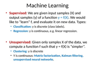
2. Machine Learning
• Supervised: We are given input samples (X) and
output samples (y) of a function y = f(X). We would
like to “learn” f, and evaluate it on new data. Types:
• Classification: y is discrete (class labels).
• Regression: y is continuous, e.g. linear regression.
• Unsupervised: Given only samples X of the data, we
compute a function f such that y = f(X) is “simpler”.
• Clustering: y is discrete
• Y is continuous: Matrix factorization, Kalman filtering,
unsupervised neural networks.

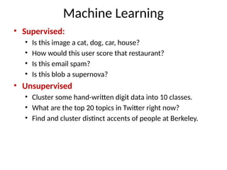
3. Machine Learning
• Supervised:
• Is this image a cat, dog, car, house?
• How would this user score that restaurant?
• Is this email spam?
• Is this blob a supernova?
• Unsupervised
• Cluster some hand-written digit data into 10 classes.
• What are the top 20 topics in Twitter right now?
• Find and cluster distinct accents of people at Berkeley.

4. Techniques
• Supervised Learning:
• kNN (k Nearest Neighbors)
• Linear Regression
• Naïve Bayes
• Logistic Regression
• Support Vector Machines
• Random Forests
• Unsupervised Learning:
• Clustering
• Factor analysis
• Topic Models

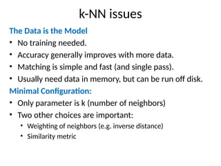
6. k-NN issues
The Data is the Model
• No training needed.
• Accuracy generally improves with more data.
• Matching is simple and fast (and single pass).
• Usually need data in memory, but can be run off disk.
Minimal Configuration:
• Only parameter is k (number of neighbors)
• Two other choices are important:
• Weighting of neighbors (e.g. inverse distance)
• Similarity metric

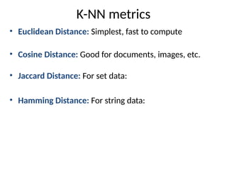
7. K-NN metrics
• Euclidean Distance: Simplest, fast to compute
• Cosine Distance: Good for documents, images, etc.
• Jaccard Distance: For set data:
• Hamming Distance: For string data:

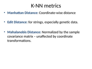
8. K-NN metrics
• Manhattan Distance: Coordinate-wise distance
• Edit Distance: for strings, especially genetic data.
• Mahalanobis Distance: Normalized by the sample
covariance matrix – unaffected by coordinate
transformations.

9. Linear Regression
We want to find the best line (linear function y=f(X)) to
explain the data.
X
y

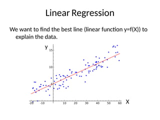
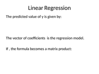
10. Linear Regression
The predicted value of y is given by:
The vector of coefficients is the regression model.
If , the formula becomes a matrix product:

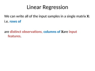
11. Linear Regression
We can write all of the input samples in a single matrix X:
i.e. rows of
are distinct observations, columns of Xare input
features.

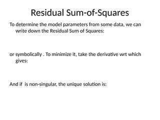
12. Residual Sum-of-Squares
To determine the model parameters from some data, we can
write down the Residual Sum of Squares:
or symbolically . To minimize it, take the derivative wrt which
gives:
And if is non-singular, the unique solution is:

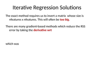
13. Iterative Regression Solutions
The exact method requires us to invert a matrix whose size is
nfeatures x nfeatures. This will often be too big.
There are many gradient-based methods which reduce the RSS
error by taking the derivative wrt
which was

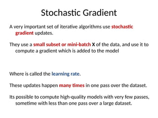
14. Stochastic Gradient
A very important set of iterative algorithms use stochastic
gradient updates.
They use a small subset or mini-batch X of the data, and use it to
compute a gradient which is added to the model
Where is called the learning rate.
These updates happen many times in one pass over the dataset.
Its possible to compute high-quality models with very few passes,
sometime with less than one pass over a large dataset.

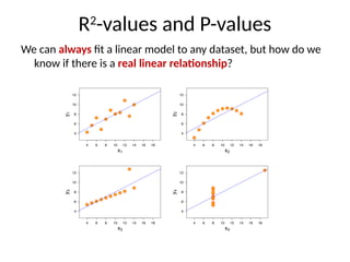
15. R2
-values and P-values
We can always fit a linear model to any dataset, but how do we
know if there is a real linear relationship?

16. R2
-values and P-values
Approach: Use a hypothesis test. The null hypothesis is that there
is no linear relationship (β = 0).
Statistic: Some value which should be small under the null
hypothesis, and large if the alternate hypothesis is true.
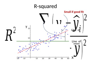
R-squared: a suitable statistic. Let be a predicted value, and be
the sample mean. Then the R-squared statistic is
And can be described as the fraction of the total variance not
explained by the model.

17. R-squared
𝑅
2
=1−
∑(𝑦𝑖−^
𝑦𝑖)2
∑(𝑦𝑖−𝑦)
2
X
y
Line of
Line of
Small if good fit

18. R2
-values and P-values
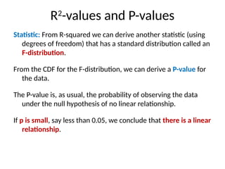
Statistic: From R-squared we can derive another statistic (using
degrees of freedom) that has a standard distribution called an
F-distribution.
From the CDF for the F-distribution, we can derive a P-value for
the data.
The P-value is, as usual, the probability of observing the data
under the null hypothesis of no linear relationship.
If p is small, say less than 0.05, we conclude that there is a linear
relationship.

19. Clustering – Why?
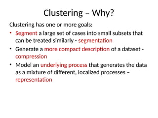
Clustering has one or more goals:
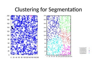
• Segment a large set of cases into small subsets that
can be treated similarly - segmentation
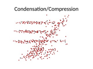
• Generate a more compact description of a dataset -
compression
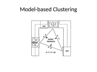
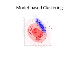
• Model an underlying process that generates the data
as a mixture of different, localized processes –
representation

20. Clustering – Why?
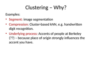
Examples:
• Segment: image segmentation
• Compression: Cluster-based kNN, e.g. handwritten
digit recognition.
• Underlying process: Accents of people at Berkeley
(??) – because place of origin strongly influences the
accent you have.

21. Stereotypical Clustering
Note: Points are samples plotted in feature space, e.g. 10,000-
dimensional space for 100x100 images.

22. Model-based Clustering

23. Model-based Clustering

24. Clustering for Segmentation

25. Condensation/Compression

26. “Cluster Bias”
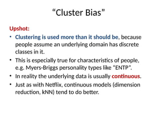
Upshot:
• Clustering is used more than it should be, because
people assume an underlying domain has discrete
classes in it.
• This is especially true for characteristics of people,
e.g. Myers-Briggs personality types like “ENTP”.
• In reality the underlying data is usually continuous.
• Just as with Netflix, continuous models (dimension
reduction, kNN) tend to do better.

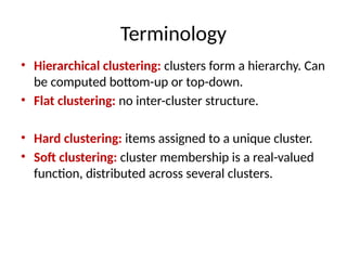
27. Terminology
• Hierarchical clustering: clusters form a hierarchy. Can
be computed bottom-up or top-down.
• Flat clustering: no inter-cluster structure.
• Hard clustering: items assigned to a unique cluster.
• Soft clustering: cluster membership is a real-valued
function, distributed across several clusters.

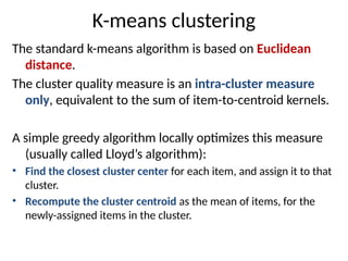
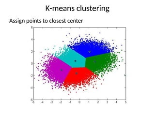
28. K-means clustering
The standard k-means algorithm is based on Euclidean
distance.
The cluster quality measure is an intra-cluster measure
only, equivalent to the sum of item-to-centroid kernels.
A simple greedy algorithm locally optimizes this measure
(usually called Lloyd’s algorithm):
• Find the closest cluster center for each item, and assign it to that
cluster.
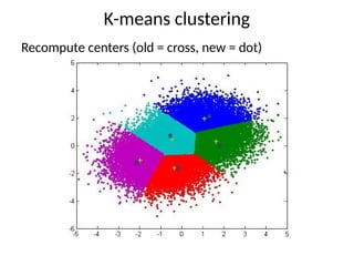
• Recompute the cluster centroid as the mean of items, for the
newly-assigned items in the cluster.

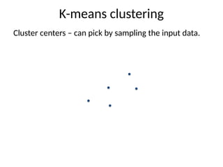
29. Cluster centers – can pick by sampling the input data.
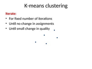
K-means clustering

30. K-means clustering
Assign points to closest center

31. K-means clustering
Recompute centers (old = cross, new = dot)

32. Iterate:
• For fixed number of iterations
• Until no change in assignments
• Until small change in quality
K-means clustering

33. K-means properties
• It’s a greedy algorithm with random setup – solution isn’t
optimal and varies significantly with different initial points.
• Very simple convergence proofs.
• Performance is O(nk) per iteration, not bad and can be
heuristically improved.
n = total features in the dataset, k = number clusters
• Many generalizations, e.g.
• Fixed-size clusters
• Simple generalization to m-best soft clustering
• As a “local” clustering method, it works well for data
condensation/compression.