SlideShare a Scribd company logo
1 of 78
Download to read offline
1
Data Mining Main Tasks
DM Task: Predictive Modeling
• A predictive model makes a prediction/forecast about
values of data using known results found from different
historical data
– Prediction Methods use existing variables to predict unknown
or future values of other variables.
• Predict one variable Y given a set of other variables X.
Here X could be an n-dimensional vector
– In effect this is function approximation through learning the
relationship between Y and X
• Many, many algorithms for predictive modeling in
statistics and machine learning, including
– Classification, regression, etc.
• Often the emphasis is on predictive accuracy, less
emphasis on understanding the model 2
3
• Classification
– Predicts categorical class labels (discrete or nominal)
– Classifies data (constructs a model) based on the
training set and the values (class labels) in a
classifying attribute and uses it in classifying new data
• Numeric Prediction
– Models continuous-valued functions,
– i.e., predicts unknown or missing values
Prediction Problems:
Classification vs. Numeric Prediction
Models and Patterns
• Model = abstract representation of a given
training data
e.g., very simple linear model structure
Y = a X + b
– a and b are parameters determined from the data
– Y = aX + b is the model structure
– Y = 0.9X + 0.3 is a particular model
• Pattern represents “local structure” in a dataset
–E.g., if X>x then Y >y with probability p
5
x f(x)
1 1
2 4
3 9
4 16
5 ?
• Example: Given a finite sample, <x,f(x)> pairs, create a
model that can hold for future values?
✓To guess the true function f, find some pattern (called a
hypothesis) in the training examples, and assume that the
pattern will hold for future examples too.
Predictive Modeling: Customer Scoring
• Example: a bank has a database of 1 million past
customers, 10% of whom took out mortgages
• Use machine learning to rank new customers as a function
of p(mortgage | customer data)
• Customer data
– History of transactions with the bank
– Other credit data (obtained from Experian, etc)
– Demographic data on the customer or where they live
• Techniques
– Binary classification: logistic regression, decision trees,
etc
– Many, many applications of this nature 6
Classification
• Example: Credit scoring
– Differentiating between low-risk and high-risk customers from
their income and savings
Discriminant rule: IF income > θ1 AND savings > θ2
THEN low-risk
ELSE high-risk
Predictive Modeling: Fraud Detection
• Credit card fraud detection
– Credit card losses in the US are over 1 billion $ per year
– Roughly 1 in 50 transactions are fraudulent
• Approach
– For each transaction estimate p(fraudulent | transaction)
– Model is built on historical data of known fraud/non-fraud
– High probability transactions investigated by fraud police
• Example:
– Fair-Isaac/HNC’s fraud detection software based on neural
networks, led to reported fraud decreases of 30 to 50%
(http://www.fairisaac.com/fairisaac)
• Issues
– Significant feature engineering/preprocessing
– false alarm rate vs. missed detection – what is the tradeoff?
8
DM Task: Descriptive Modeling
9
3.3 3.4 3.5 3.6 3.7 3.8 3.9 4
3.7
3.8
3.9
4
4.1
4.2
4.3
4.4
Red Blood Cell Volume
Red
Blood
Cell
Hemoglobin
Concentration
EM ITERATION 25
• Goal is to build a “descriptive” model that models the underlying
observation
– e.g., a model that could simulate the data if needed
• Description Methods find human-interpretable patterns that
describe and find natural groupings of the data.
• Methods used in descriptive modeling are: clustering,
summarization, association rule discovery, etc.
• Descriptive model identifies
patterns or relationship in data
– Unlike the predictive model, a
descriptive model serves as a way
to explore the properties of the
data examined, not to predict new
properties
Example of Descriptive Modeling
• goal: learn directed relationships among p variables
• techniques: directed (causal) graphs
• challenge: distinguishing between correlation and causation
– Example: Do yellow fingers cause lung cancer?
cancer
yellow fingers
?
smoking hidden cause: smoking
10
Pattern (Association Rule) Discovery
• Goal is to discover interesting “local” patterns
(sequential patterns) in the data rather than to
characterize the data globally
– Also called link analysis (uncovers relationships
among data)
• Given market basket data we might discover that
– If customers buy wine and bread then they buy
cheese with probability 0.9
• Methods used in pattern discovery include:
– Association rules, Sequence discovery, etc.
11
Example of Pattern Discovery
• Example in retail: Customer transactions to consumer behavior:
– People who bought “Da Vinci Code” also bought “The Five
People You Meet in Heaven” (www.amazon.com)
• Example: football player behavior
– If player A is in the game, player B’s scoring rate increases
from 25% chance per game to 95% chance per game
• What about the following?
12
ADACABDABAABBDDBCADDDDBCDDBCCBBCCDADADAADABDBBDABABBCDDDCDDABDC
BBDBDBCBBABBBCBBABCBBACBBDBAACCADDADBDBBCBBCCBBBDCABDDBBADDBBBBCC
ACDABBABDDCDDBBABDBDDBDDBCACDBBCCBBACDCADCBACCADCCCACCDDADCBCAD
ADBAACCDDDCBDBDCCCCACACACCDABDDBCADADBCBDDADABCCABDAACABCABACB
DDDCBADCBDADDDDCDDCADCCBBADABBAAADAAABCCBCABDBAADCBCDACBCABABC
CBACBDABDDDADAABADCDCCDBBCDBDADDCCBBCDBAADADBCAAAADBDCADBDBBBC
DCCBCCCDCCADAADACABDABAABBDDBCADDDDBCDDBCCBBCCDADADACCCDABAABBC
BDBDBADBBBBCDADABABBDACDCDDDBBCDBBCBBCCDABCADDADBACBBBCCDBAAADDD
BDDCABACBCADCDCBAAADCADDADAABBACCBB
13
Supervised vs. Unsupervised Learning
• Supervised learning (classification)
– Supervision: The training data (observations, measurements,
etc.) are accompanied by labels indicating the class of the
observations
– New data is classified based on the training set
• Unsupervised learning (clustering)
– The class labels of training data is unknown
– Given a set of measurements, observations, etc. with the
aim of establishing the existence of classes or clusters in the
data
Basic Data Mining algorithms
• Classification (which is also called Supervised learning) maps data
into predefined groups or classes to enhance the prediction
process
• Clustering (which is also called Unsupervised learning )
groups similar data together into clusters.
– is used to find appropriate groupings of elements for a set of
data.
– Unlike classification, clustering is a kind of undirected knowledge
discovery or unsupervised learning; that is, there is no target field,
and the relationship among the data is identified by bottom-up
approach.
• Association Rule (is also known as market basket analysis)
– It discovers interesting associations between attributes contained
in a database.
– Based on frequency counts of the number of items occur in the
event, association rule tells if item X is a part of the event, then
what is the percentage of item Y is also part of the event.
14
Classification
15
Classification: Definition
• Classification is a data mining (machine learning) technique
used to predict group membership for data instances.
• Given a collection of records (training set), each record
contains a set of attributes, one of the attributes is the class.
– Find a model for class attribute as a function of the values of
other attributes.
• Goal: previously unseen records should be assigned a class as
accurately as possible. A test set is used to determine the
accuracy of the model.
– Usually, the given data set is divided into training and test sets,
with training set used to build the model and test set used to
validate it.
• For example, one may use classification to predict whether the
weather on a particular day will be “sunny”, “rainy” or “cloudy”.
16
17
Classification—A Two-Step Process
• Model construction: describing a set of predetermined classes
– Each tuple/sample is assumed to belong to a predefined class, as
determined by the class label attribute
– The set of tuples used for model construction is training set
– The model is represented as classification rules, decision trees,
or mathematical formula
• Model usage: for classifying future or unknown objects
– Estimate accuracy of the model
• The known label of test sample is compared with the
classified result from the model
• Accuracy rate is the percentage of test set samples that are
correctly classified by the model
• Test set is independent of training set
– If the accuracy is acceptable, use the model to classify data
tuples whose class labels are not known
Illustrating Classification Task
Apply
Model
Induction
Deduction
Learn
Model
Model
Tid Attrib1 Attrib2 Attrib3 Class
1 Yes Large 125K No
2 No Medium 100K No
3 No Small 70K No
4 Yes Medium 120K No
5 No Large 95K Yes
6 No Medium 60K No
7 Yes Large 220K No
8 No Small 85K Yes
9 No Medium 75K No
10 No Small 90K Yes
10
Tid Attrib1 Attrib2 Attrib3 Class
11 No Small 55K ?
12 Yes Medium 80K ?
13 Yes Large 110K ?
14 No Small 95K ?
15 No Large 67K ?
10
Test Set
Learning
algorithm
Training Set
Confusion Matrix for Performance Evaluation
• Most widely-used metric is measuring Accuracy of the
system :
• Other metric for performance evaluation are Precision,
Recall & F-Measure
PREDICTED CLASS
ACTUAL
CLASS
Class=Yes Class=No
Class=Yes a
(TP)
b
(FP)
Class=No c
(FP)
d
(TP)
100
*
Accuracy
FP
TP
TP
d
c
b
a
d
a
+
=
+
+
+
+
=
Classification methods
• Goal: Predict class Ci = f(x1, x2, .. xn)
• There are various classification methods. Popular
classification techniques include the following.
– K-nearest neighbor
– Decision tree classifier: divide decision space into
piecewise constant regions.
– Neural networks: partition by non-linear
boundaries
– Bayesian network: a probabilistic model
– Support Vector Machine (SVM)
20
K-Nearest Neighbors
• K-nearest neighbor is a supervised learning algorithm where
the result of new instance query is classified based on
majority of K-nearest neighbor category.
• The purpose of this algorithm is to classify a new object based
on attributes and training samples: (xn, f(xn)), n=1..N.
• Given a query point, we find K number of objects or (training
points) closest to the query point.
– The classification is using majority vote among the classification
of the K objects.
– K Nearest neighbor algorithm used neighborhood classification
as the prediction value of the new query instance.
• K nearest neighbor algorithm is very simple. It works based on
minimum distance from the query instance to the training
samples to determine the K-nearest neighbors.
21
How to compute K-Nearest Neighbor (KNN)
Algorithm?
• Determine parameter K = number of nearest neighbors
• Calculate the distance between the query-instance and all
the training samples
– We can use Euclidean distance
• Sort the distance and determine nearest neighbors based
on the Kth minimum distance
• Gather the category of the nearest neighbors
• Use simple majority of the category of nearest neighbors
as the prediction value of the query instance
– Any ties can be broken at random.
23
K Nearest Neighbors: Key issues
The key issues involved in training KNN model includes
• Setting the variable K - Number of nearest neighbors
–The numbers of nearest neighbors (K) should be based on cross
validation over a number of K setting.
–When k=1 is a good baseline model to benchmark against.
–A good rule-of-thumb is that K should be less than or equal to the
square root of the total number of training patterns.
• Setting the type of distant metric
–We need a measure of distance in order to know who are the
neighbours
–Assume that we have T attributes for the learning problem. Then
one example point x has elements xt  , t=1,…T.
–The distance between two points xi xj is often defined as the
Euclidean distance: 2
1
)
(
)
,
( 
=
−
=
D
i
Yi
Xi
Y
X
Dist
N
K 
k-Nearest Neighbors (k-NN)
▪ K-NN is an algorithm that can be used when you have a
bunch of objects that have been classified or labeled in some
way, and other similar objects that haven’t gotten
classified or labeled yet, and you want a way to
automatically label them
▪ The objects could be data scientists who have been
classified as “active” or “passive”; or people who have
been labeled as “high credit” or “low credit”; or restaurants
that have been labeled “five star,” “four star,” “three star,”
“two star,” “one star,” or if they really suck, “zero stars.”
▪ More seriously, it could be patients who have been
classified as “high cancer risk” or “low cancer risk.”
24
25
K-NN
• K-NN is a Supervised machine learning while K-
NN is a classification or regression machine
learning algorithm
• K-NN is a lazy learner while K-Means is
an eager learner. An eager learner has a model
fitting that means a training step but a lazy
learner does not have a training phase.
• K-NN performs much better if all of the data
have the same scale (Labelled Data) but this is
not true for K-means.
26
K-Nearest Neighbor(K-NN)
K-Nearest Neighbor Classification (KNN)
• Example with credit scores:
• Say you have the age, income, and a credit category
of high or low for a bunch of people and you want to
use the age and income to predict the credit label of
“high” or “low” for a new person.
• For example, here are the first few rows of a dataset,
with income represented in thousands
27
K-Nearest Neighbor Classification (KNN)
• What if a new guy comes in who is 57 years
old and who makes $37,000? What’s his
likely credit rating label?
28
Distance Function Measurements
29
Hamming Distance
• For category variables, Hamming distance
can be used.
30
K-Nearest-Neighbors
31
What is the most possible label for C?
c
32
Solution: Looking for the nearest K neighbors of C.
Take the majority label as C’s label Let’s suppose K = 3:
What is the most possible label for C?
C
33
• The 3 nearest points to C are: a, a and o.
• Therefore, the most possible label for C is a.
Example
• We have data from the questionnaires survey (to ask
people opinion) and objective testing with two attributes
(acid durability and strength) to classify whether a special
paper tissue is good or not. Here is four training samples.
• Now the factory produces a new paper tissue that pass
laboratory test with X1 = 3 and X2 = 7.
– Without undertaking another expensive survey, guess the
goodness of the new tissue?
– Use squared Euclidean distance for similarity measurement.
X1 = Acid Durability (seconds) X2 = Strength (kg/m2) Y = Classification
7 7 Bad
7 4 Bad
3 4 Good
1 4 Good
Solution
X1 = Acid
Durability
(seconds)
X2 =
Strength
(kg/m2)
Square Distance
to query instance
(3, 7)
Rank
minimum
distance
Is it
included
in 3-
NNs?
Y =
Category
of NN
7 7 3 Yes Bad
7 4 4 No -
3 4 1 Yes Good
1 4 2 Yes Good
• Use simple majority of the category of nearest neighbors as the prediction value of
the query instance. We have 2 good and 1 bad, since 2>1 then we conclude that a
new paper tissue that pass laboratory test with X1 = 3 and X2 = 7 is included in
Good category.
37
KNNs: advantages & Disadvantages
• Advantage
– Nonparametric architecture
– Simple
– Powerful
– Requires no training time
• Disadvantage: Difficulties with k-nearest neighbour
algorithms
– Memory intensive: just store the training examples
• when a test example is given then find the closest matches
– Classification/estimation is slow
– Have to calculate the distance of the test case from all training
cases
– There may be irrelevant attributes amongst the attributes –
curse of dimensionality
Decision Tree
39
Decision Trees
• Decision tree constructs a tree where internal nodes are simple
decision rules on one or more attributes and leaf nodes are
predicted class labels.
✓Given an instance of an object or situation, which is specified by a
set of properties, the tree returns a "yes" or "no" decision about
that instance.
Attribute_1
Attribute_2 Attribute_2
value-1
value-2
value-3
Class1
Class1
Class2 Class2
Class1
value-5 value-4 value-6 value-7
Choosing the Splitting Attribute
• At each node, the best attribute is selected for splitting the
training examples using a Goodness function
– The best attribute is the one that separate the classes of the
training examples faster such that it results in the smallest tree
• Typical goodness functions:
– information gain, information gain ratio, and Gini index
•Information Gain
–Select the attribute with the highest information gain, that create
small average disorder
• First, compute the disorder using Entropy; the expected
information needed to classify objects into classes
• Second, measure the Information Gain; to calculate by how
much the disorder of a set would reduce by knowing the value
of a particular attribute.
Entropy
)
(
log
log
)
,
( 2
2 S
Entropy
n
n
n
n
n
n
n
n
n
n
D =
−
−
= −
−
+
+
−
+
• The Entropy measures the disorder of a set S containing a total of
n examples of which n+ are positive and n- are negative and it is
given by:
• Some useful properties of the Entropy:
– D(n,m) = D(m,n)
– D(0,m) = D(m,0) = 0
✓D(S)=0 means that all the examples in S have the same
class
– D(m,m) = 1
✓D(S)=1 means that half the examples in S are of one
class and half are in the opposite class
Information Gain
• The Information Gain measures the expected reduction
in entropy due to splitting on an attribute A
Parent Node, S is split into k partitions;
ni is number of records in partition i
• Information Gain: Measures Reduction in Entropy
achieved because of the split. Choose the split that
achieves most reduction (maximizes GAIN)






−
= 
=
k
i
i
split i
Entropy
n
n
S
Entropy
GAIN
1
)
(
)
(
Example 1: The problem of “Sunburn”
• You want to predict whether another person is likely to get sunburned
if he/she is back to the beach. How can you do this?
• Data Collected: predict based on the observed properties of the
people
Name Hair Height Weight Lotion Result
Sarah Blonde Average Light No Sunburned
Dana Blonde Tall Average Yes None
Alex Brown Short Average Yes None
Annie Blonde Short Average No Sunburned
Emily Red Average Heavy No Sunburned
Pete Brown Tall Heavy No None
John Brown Average Heavy No None
Kate Blonde Short Light Yes None
Attribute Selection by Information Gain to
construct the optimal decision tree
954
.
0
8
5
log
8
5
8
3
log
8
3
)
5
,
3
( 2
2 =
−
−
=
= −
+
D
D({ “Sarah”,“Dana”,“Alex”,“Annie”, “Emily”,“Pete”,“John”,“Katie”})
• Entropy: The Disorder of Sunburned
Which decision variable minimises the
disorder?
Test Average Disorder of the other attributes
Hair 0.50
height 0.69
weight 0.94
lotion 0.61
• Which decision variable maximises the Info Gain then?
• Remember it’s the one which minimises the average disorder.
✓ Gain(hair) = 0.954 - 0.50 = 0.454
✓ Gain(height) = 0.954 - 0.69 =0.264
✓ Gain(weight) = 0.954 - 0.94 =0.014
✓ Gain (lotion) = 0.954 - 0.61 =0.344
The best decision tree?
?
is_sunburned
Alex
Pete
John
Emily
Sunburned = Sarah, Annie, None
= Dana, Katie
Hair colour
brown
blonde
red
• Once we have finished with hair colour we then need to calculate
the remaining branches of the decision tree.
• Which attributes is better to classify the remaining ?
The best Decision Tree
Sarah,
Annie
is_sunburned
Alex,
Pete,
John
Emily
Dana,
Katie
Hair colour
Lotion used
blonde
red
brown
no yes
• This is the simplest and optimal one possible and it makes a lot of
sense.
• It classifies 4 of the people on just the hair colour alone.
Sunburn sufferers are ...
• You can view Decision Tree as an IF-THEN_ELSE
statement which tells us whether someone will suffer
from sunburn.
If (Hair-Colour=“red”) then
return (sunburned = yes)
else if (hair-colour=“blonde” and lotion-
used=“No”) then
return (sunburned = yes)
else
return (false)
53
Exercise: Decision Tree for “buy computer or not”. Use the
training Dataset given below to construct decision tree
age income student credit_rating buys_computer
<=30 high no fair no
<=30 high no excellent no
31…40 high no fair yes
>40 medium no fair yes
>40 low yes fair yes
>40 low yes excellent no
31…40 low yes excellent yes
<=30 medium no fair no
<=30 low yes fair yes
>40 medium yes fair yes
<=30 medium yes excellent yes
31…40 medium no excellent yes
31…40 high yes fair yes
>40 medium no excellent no
54
Output: A Decision Tree for “buys_computer”
age?
overcast
student? credit rating?
<=30 >40
no yes yes
yes
31..40
fair
excellent
yes
no
Why decision tree induction in DM?
Cons
- Cannot handle complicated
relationship between features
- Simple decision boundaries
- Problems with lots of missing
data
Pros
+ Reasonable training time
+ Fast application
+ Easy to interpret
+ Easy to implement
+ Can handle large number of
features
56
• Relatively faster learning speed (than other classification methods)
• Convertible to simple and easy to understand classification if-then-
else rules
• Comparable classification accuracy with other methods
• Does not require any prior knowledge of data distribution, works
well on noisy data.
Bayesian Learning
Why Bayesian Classification?
• Provides practical learning algorithms
– Probabilistic learning: Calculate explicit probabilities
for hypothesis. E.g. Naïve Bayes
• Prior knowledge and observed data can be combined
– Incremental: Each training example can incrementally
increase/decrease the probability that a hypothesis is correct.
• It is a generative (model based) approach, which offers a
useful conceptual framework
– Probabilistic prediction: Predict multiple hypotheses, weighted
by their probabilities. E.g. sequences could also be classified,
based on a probabilistic model specification
– Any kind of objects can be classified, based on a probabilistic
model specification
CONDITIONAL PROBABILITY
• Probability : How likely is it that an event will happen?
• Sample Space S
– An event A and C are a subset of S
• P(C / A)- Probability that event C occurs given that event
A has already occurred.
Example of conditional probability:
• There are 2 baskets. B1 has 2 red ball and 5 blue ball.
B2 has 4 red ball and 3 blue ball.
– Find probability of picking a red ball from basket 1?
P(red ball | basket 1) =
– What about P(basket2 | red ball) ?
)
(
)
,
(
)
|
(
A
P
C
A
P
A
C
P =
Bayes Classifier
• A probabilistic framework for solving classification problems
• Bayes theorem:
• Example of Bayes Theorem
– Given: A doctor knows that meningitis causes stiff neck 50% of
the time. Prior probability of any patient having meningitis is
1/50. Prior probability of any patient having stiff neck is 1/20. If
a patient has stiff neck, what’s the probability he/she has
meningitis?
)
(
)
(
)
|
(
)
|
(
A
P
C
P
C
A
P
A
C
P =
)
(
)
,
(
)
|
(
C
P
C
A
P
C
A
P =
)
(
)
,
(
)
|
(
A
P
C
A
P
A
C
P =
Bayes Theorem
• Example 2: A medical cancer diagnosis problem. There are 2
possible outcomes of a diagnosis: +ve, -ve.
We know 0.8% of world population has cancer. Test gives correct
+ve result 98% of the time and gives correct –ve result 97% of
the time. If a patient’s test returns +ve, should we diagnose the
patient as having cancer?
P(cancer) = 0.008 p(no-cancer) = 0.992
P(+ve|cancer) = 0.98 P(-ve|cancer) = 0.02
P(+ve|no-cancer) = 0.03 P(-ve|no-cancer) = 0.97
Using Bayes Formula:
– P(cancer|+ve) = P(+ve|cancer)xP(cancer) / P(+ve)
= 0.98 x 0.008 = 0.0078 / P(+ve)
– P(no-cancer|+ve) = P(+ve|no-cancer)xP(no-cancer) / P(+ve)
= 0.03 x 0.992 = 0.0298 / P(+ve)
So, the patient most likely does not have cancer.
General Bayes Theorem
• Consider each attribute and class label as random variables
• Given a record with attributes (A1, A2,…,An)
– Goal is to predict class C
– Specifically, we want to find the value of C that maximizes P(C|
A1, A2,…,An )
• Can we estimate P(C| A1, A2,…,An ) directly from data?
– Approach: compute the posterior probability P(C | A1, A2, …,
An) for all values of C using the Bayes theorem
– Choose value of C that maximizes: P(C | A1, A2, …, An)
– Equivalent to choosing value of C that maximizes
P(A1, A2, …, An|C) P(C)
• How to estimate P(A1, A2, …, An | C )?
)
(
)
(
)
|
(
)
|
(
2
1
2
1
2
1
n
n
n
A
A
A
P
C
P
C
A
A
A
P
A
A
A
C
P


 =
Naïve Bayes Classifier
• Assume independence among attributes Ai when class is
given:
– P(A1, A2, …, An |C) = P(A1| Cj) P(A2| Cj)… P(An| Cj)
– Can estimate P(Ai| Cj) for all Ai and Cj.
– New point is classified to Cj if P(Cj)  P(Ai| Cj) is
maximal.

=
i
j
i
j
j
Bayes
Naive C
A
P
C
P
C )
|
(
)
(
max
arg
Example. ‘Play Tennis’ data
Day Outlook Temperature Humidity Wind Play Tennis
Day1 Sunny Hot High Weak No
Day2 Sunny Hot High Strong No
Day3 Overcast Hot High Weak Yes
Day4 Rain Mild High Weak Yes
Day5 Rain Cool Normal Weak Yes
Day6 Rain Cool Normal Strong No
Day7 Overcast Cool Normal Strong Yes
Day8 Sunny Mild High Weak No
Day9 Sunny Cool Normal Weak Yes
Day10 Rain Mild Normal Weak Yes
Day11 Sunny Mild Normal Strong Yes
Day12 Overcast Mild High Strong Yes
Day13 Overcast Hot Normal Weak Yes
Day14 Rain Mild High Strong No
• Suppose that you have a free afternoon and you are thinking whether
or not to go and play tennis, How you do that?
✓Based on the following training data, predict when this player will
Play Tennis?
Naive Bayes Classifier
• Given a training set, we can compute the probabilities
Outlook P N Humidity P N
sunny 2/9 3/5 high 3/9 4/5
overcast 4/9 0 normal 6/9 1/5
rain 3/9 2/5
Tempreature Windy
hot 2/9 2/5 Strong 3/9 3/5
mild 4/9 2/5 Weak 6/9 2/5
cool 3/9 1/5
P(P) = 9/14
P(N) = 5/14
Where, P(P) is the probability of playing tennis =
Yes and P(n) is the probability of playing tennis =
No
• Based on the model created, predict Play Tennis or Not for the
following unseen sample
(Outlook=Sunny, Temperature=Cool, Humidity=High, Wind=Strong)
• Working:
)
|
(
)
|
(
)
|
(
)
|
(
)
(
max
arg
)
|
(
)
(
max
arg
]
,
[
]
,
[
C
strong
Wind
P
C
high
Hum
P
C
cool
Temp
P
C
sunny
Outl
P
C
P
C
a
P
C
P
C
no
yes
C
t
t
no
yes
C
NB
=
=
=
=
=
=



no
PlayTennis
answer
no
strong
P
no
high
P
no
cool
P
no
sunny
P
no
P
yes
strong
P
yes
high
P
yes
cool
P
yes
sunny
P
yes
P
=

=
=
:
)
|
(
)
|
(
)
|
(
)
|
(
)
(
0053
.
0
)
|
(
)
|
(
)
|
(
)
|
(
)
(
0.0206
Play-tennis example
• More example: What if the following test data is given:
X= <Outlook=rain, Temperature=hot, Humidity=high, Wind=weak>
Exercise: Naïve Bayes Classifier
Name
Give
Birth
Can
Fly
Live in
Water
Have
Legs Class
human yes no no yes mammals
python no no no no non-mammals
salmon no no yes no non-mammals
whale yes no yes no mammals
frog no no sometimes yes non-mammals
komodo no no no yes non-mammals
bat yes yes no yes mammals
pigeon no yes no yes non-mammals
cat yes no no yes mammals
leopard shark yes no yes no non-mammals
turtle no no sometimes yes non-mammals
penguin no no sometimes yes non-mammals
porcupine yes no no yes mammals
eel no no yes no non-mammals
salamander no no sometimes yes non-mammals
gila monster no no no yes non-mammals
platypus no no no yes mammals
owl no yes no yes non-mammals
dolphin yes no yes no mammals
eagle no yes no yes non-mammals
Give Birth Can Fly Live in Water Have Legs Class
yes no yes no ?
0027
.
0
20
13
004
.
0
)
(
)
|
(
021
.
0
20
7
06
.
0
)
(
)
|
(
0042
.
0
13
4
13
3
13
10
13
1
)
|
(
06
.
0
7
2
7
2
7
6
7
6
)
|
(
=

=
=

=
=



=
=



=
N
P
N
A
P
M
P
M
A
P
N
A
P
M
A
P
A: attributes
M: mammals
N: non-mammals
P(A|M)P(M) > P(A|N)P(N)
=> Mammals
Neural Network
70
71
Brain vs. Machine
• The Brain
– Pattern Recognition
– Association
– Complexity
– Noise Tolerance
• The Machine
– Calculation
– Precision
– Logic
72
Features of the Brain
• Ten billion (1010) neurons
✓ Neuron switching time >10-3secs
• Face Recognition ~0.1secs
• On average, each neuron has several thousand
connections
• Hundreds of operations per second
• High degree of parallel computation
• Distributed representations
• Die off frequently (never replaced)
• Compensated for problems by massive parallelism
Neural Network
• Computing systems modeled after the
brain’s networks of interconnected
processing elements (neurons)
• Interconnected processors operate in parallel and
interact with each other
• Allows the network to learn from the data it
processes
• capable of finding and differentiating
• Neural Networks can:
• Learn and adjust to new circumstances on their
own
• Take part in massive parallel processing
• Function without complete information
• Cope with huge volumes of information
• Analyze nonlinear relationships
Chapter II – Organization & IS
Neural Network classifier
• It is represented as a layered set of interconnected
processors. These processor nodes has a relationship
with the neurons of the brain. Each node has a
weighted connection to several other nodes in adjacent
layers. Individual nodes take the input received from
connected nodes and use the weights together to
compute output values.
• The inputs are fed simultaneously into the input layer.
• The weighted outputs of these units are fed into hidden
layer.
• The weighted outputs of the last hidden layer are inputs
to units making up the output layer.
75
Architecture of Neural network
• Neural networks are used to look for patterns in data, learn
these patterns, and then classify new patterns & make forecasts
• A network with the input and output layer only is called single-
layered neural network. Whereas, a multilayer neural network
is a generalized one with one or more hidden layer.
– A network containing two hidden layers is called a three-layer neural
network, and so on.
Hidden
nodes
Output
nodes
x1
x2
x3
x1
x2
x3
w1
w2
w3
y
n
i
i
i
e
y
x
w
o
−
=
+
=
= 
1
1
)
(
)
(
1


Single layered NN Multilayer NN
Input
nodes
A Multilayer Neural Network
• INPUT: records with class attribute with
normalized attributes values.
–INPUT VECTOR: X = { x1, x2, …. xm},
where m is the number of attributes.
–INPUT LAYER – there are as many nodes as
class attributes i.e. as the length of the input
vector.
• HIDDEN LAYER – neither its input nor its
output can be observed from outside.
–The number of nodes in the hidden layer
and the number of hidden layers depends on
implementation.
Input layer
Hidden layer
Output layer
• OUTPUT LAYER – corresponds to the class attribute.
–There are as many nodes as classes (values of the class
attribute).
–Ok, where k= 1, 2,.. n, where n is number of classes
Hidden layer: Neuron with Activation
• The neuron is the basic information processing unit of a
NN. It consists of:
1 A set of links, describing the neuron inputs, with
weights W1, W2, …, Wm
2. An adder function (linear combiner) for computing the
weighted sum of the inputs (real numbers):
3. Activation function (also called squashing function):
for limiting the output behavior of the neuron.

=
=
m
1
j
jx
w
y
j
)
(y
y b
+
=
Activation Functions
•(a) is a step function or threshold function (hardlimiting):
•(b) is a sigmoid function: 1/(1+e-x)
•Changing the bias weight W0,i moves the threshold location
–Bias helps the neural network to be more flexible since it adjust
the activation function left-or-right, making it centered on some
other value than x = 0. To this effect an additional node is added
to the input layer, with its constant input; say, 1 or -1, … When this
is multiplied by the weights of the hidden layer, it provides a bias
(DC offset) to activation function.
Two Topologies of neural network
• NN can be designed in a feed forward or recurrent
manner
• In a feed forward neural network connections
between the units do not form a directed cycle.
– In this network, the information moves in only one
direction, forward, from the input nodes, through the
hidden nodes (if any) & to the output nodes. There are
no cycles or loops or no feedback connections are
present in the network, that is, connections extending
from outputs of units to inputs of units in the same layer
or previous layers.
• In recurrent networks data circulates back &
forth until the activation of the units is
stabilized
– Recurrent networks have a feedback loop where data
can be fed back into the input at some point before
it is fed forward again for further processing and
final output.
81
Training the neural network
• The purpose is to learn to generalize using a set of sample
patterns where the desired output is known.
• Back Propagation is the most commonly used method for
training multilayer feed forward NN.
– Back propagation learns by iteratively processing a set of training
data (samples).
– For each sample, weights are modified to minimize the error
between the desired output and the actual output.
• After propagating an input through the network, the error
is calculated and the error is propagated back through
the network while the weights are adjusted in order to
make the error smaller.
82
Training Algorithm
•The applied learning algorithm is as follows
–Initialize the weights and threshold to small random numbers.
–Present a vector x to the neuron inputs and calculate the output
using the adder function.
–Apply the activation function such that
–Update the weights according to the error.
j
T
j
j x
y
y
W
W *
)
(
* −
+
= 

=
=
m
1
j
jx
w
y
j







= 0
y
if
1
0
y
if
0
y
ANN Training Example
• Training – epoch 1:
y1 = 0.92*0 + 0.62*0 – 0.22 = -0.22 → y = 0
y2 = 0.92*1 + 0.62*0 – 0.22 = 0.7 → y =1
W1(1) = 0.92 + 0.1 * (0 – 1) * 1 = 0.82
W2(1) = 0.62 + 0.1 * (0 – 1) * 0 = 0.62
W0(1) = 0.22 + 0.1 * (0 – 1) * (-1)= 0.32
y3 = 0.82*0 + 0.62*1 – 0.32 = 0.3 → y = 1
y4 = 0.82*1 + 0.62*1 – 0.32 = 1.12 → y =1
X
Bias 1st input
(x1)
2nd input
(x2)
Target
output
-1 0 0 0
-1 1 0 0
-1 0 1 1
-1 1 1 1
Given the following two inputs x1, x2;
find equation that helps to draw the
boundary?
• Let say we have the following initializations:
W1(0) = 0.92, W2(0) = 0.62,
W0(0) = 0.22, ή = 0.1
ANN Training Example
• Training – epoch 2:
y1 = 0.82*0 + 0.62*0 – 0.32 = -0.32 → y= 0
y2 = 0.82*1 + 0.62*0 – 0.32 = 0.5 → y= 1
W1(2) = 0.82 + 0.1 * (0 – 1) * 1 = 0.72
W2(2) = 0.62 + 0.1 * (0 – 1) * 0 = 0.62
W0(2) = 0.32 + 0.1 * (0 – 1) * (-1)= 0.42
y3 = 0.72*0 + 0.62*1 – 0.42 = 0.2 → y= 1
y4 = 0.72*1 + 0.62*1 – 0.42 = 0.92 → y = 1
• Training – epoch 3:
y1 = 0.72*0 + 0.62*0 – 0.42 = -0.42 → y = 0
y2 = 0.72*1 + 0.62*0 – 0.42 = 0.4 → y = 1
W1(3) = 0.72 + 0.1 * (0 – 1) * 1 = 0.62
W2(3) = 0.62 + 0.1 * (0 – 1) * 0 = 0.62
W0(3) = 0.42 + 0.1 * (0 – 1) * (-1)= 0.52
y3 = 0.62*0 + 0.62*1 – 0.52 = 0.1→ y = 1
y4 = 0.62*1 + 0.62*1 – 0.52 = 0.72→ y = 1
X
X
ANN Training Example
• Training – epoch 4:
y1 = 0.62*0 + 0.62*0 – 0.52 = -0.52 → y = 0
y2 = 0.62*1 + 0.62*0 – 0.52 = 0.10→ y = 1
W1(4) = 0.62 + 0.1 * (0 – 1) * 1 = 0.52
W2(4) = 0.62 + 0.1 * (0 – 1) * 0 = 0.62
W0(4) = 0.52 + 0.1 * (0 – 1) * (-1)= 0.62
y3 = 0.52*0 + 0.62*1 – 0.62 = 0 → y = 0
W1(4) = 0.52 + 0.1 * (1 – 0) * 0 = 0.52
W2(4) = 0.62 + 0.1 * (1 – 0) * 1 = 0.72
W0(4) = 0.62 + 0.1 * (1 – 0) * (-1)= 0.52
y4 = 0.52*1 + 0.72*1 – 0.52 = 0.72 → y = 1
• Finally:
y1 = 0.52*0 + 0.72*0 – 0.52 = -0.52 → y = 0
y2 = 0.52*1 + 0.72*0 – 0.52 = -0.0 → y = 0
y3 = 0.52*0 + 0.72*1 – 0.52 = 0.2 → y= 1
y4 = 0.52*1 + 0.72*1 – 0.52 = 0.72 → y= 1
X
X
ANN Training Example
+ +
1
o 1
0
x2
x1
o
+ +
1
o 1
0
x2
x1
o
Pros and Cons of Neural Network
Cons
-Slow training time
- Hard to interpret & understand
the learned function (weights)
-Hard to implement: trial & error for
choosing number of nodes
Pros
+ Can learn more complicated
class boundaries
+ Fast application
+ Can handle large number of
features
Neural Network needs long time for training.
Neural Network has a high tolerance to noisy and incomplete data
Conclusion: Use neural nets only if decision-trees fail.
91
• Useful for learning complex data like handwriting, speech and
image recognition

More Related Content

Similar to Chapter 4 Classification in data sience .pdf

Types of Machine Learning- Tanvir Siddike Moin
Types of Machine Learning- Tanvir Siddike MoinTypes of Machine Learning- Tanvir Siddike Moin
Types of Machine Learning- Tanvir Siddike MoinTanvir Moin
 
Data mining an introduction
Data mining an introductionData mining an introduction
Data mining an introductionDr-Dipali Meher
 
Classification and Prediction.pptx
Classification and Prediction.pptxClassification and Prediction.pptx
Classification and Prediction.pptxSandeepAgrawal84
 
01 Introduction to Data Mining
01 Introduction to Data Mining01 Introduction to Data Mining
01 Introduction to Data MiningValerii Klymchuk
 
Unit-V Machine Learning.ppt
Unit-V Machine Learning.pptUnit-V Machine Learning.ppt
Unit-V Machine Learning.pptSharpmark256
 
The 8 Step Data Mining Process
The 8 Step Data Mining ProcessThe 8 Step Data Mining Process
The 8 Step Data Mining ProcessMarc Berman
 
It's Machine Learning Basics -- For You!
It's Machine Learning Basics -- For You!It's Machine Learning Basics -- For You!
It's Machine Learning Basics -- For You!To Sum It Up
 
Lesson 1 - Overview of Machine Learning and Data Analysis.pptx
Lesson 1 - Overview of Machine Learning and Data Analysis.pptxLesson 1 - Overview of Machine Learning and Data Analysis.pptx
Lesson 1 - Overview of Machine Learning and Data Analysis.pptxcloudserviceuit
 
Lecture 2 - Introduction to Machine Learning, a lecture in subject module Sta...
Lecture 2 - Introduction to Machine Learning, a lecture in subject module Sta...Lecture 2 - Introduction to Machine Learning, a lecture in subject module Sta...
Lecture 2 - Introduction to Machine Learning, a lecture in subject module Sta...Maninda Edirisooriya
 
Lecture 2 Data mining process.pdf
Lecture 2 Data mining process.pdfLecture 2 Data mining process.pdf
Lecture 2 Data mining process.pdfKaushik Kundu
 
Data mining chapter04and5-best
Data mining chapter04and5-bestData mining chapter04and5-best
Data mining chapter04and5-bestABDUmomo
 

Similar to Chapter 4 Classification in data sience .pdf (20)

Types of Machine Learning- Tanvir Siddike Moin
Types of Machine Learning- Tanvir Siddike MoinTypes of Machine Learning- Tanvir Siddike Moin
Types of Machine Learning- Tanvir Siddike Moin
 
Lecture 3 ml
Lecture 3 mlLecture 3 ml
Lecture 3 ml
 
Data mining
Data miningData mining
Data mining
 
Unit-1.ppt
Unit-1.pptUnit-1.ppt
Unit-1.ppt
 
Classification
ClassificationClassification
Classification
 
Data mining an introduction
Data mining an introductionData mining an introduction
Data mining an introduction
 
Classification and Prediction.pptx
Classification and Prediction.pptxClassification and Prediction.pptx
Classification and Prediction.pptx
 
01 Introduction to Data Mining
01 Introduction to Data Mining01 Introduction to Data Mining
01 Introduction to Data Mining
 
Unit-V Machine Learning.ppt
Unit-V Machine Learning.pptUnit-V Machine Learning.ppt
Unit-V Machine Learning.ppt
 
The 8 Step Data Mining Process
The 8 Step Data Mining ProcessThe 8 Step Data Mining Process
The 8 Step Data Mining Process
 
It's Machine Learning Basics -- For You!
It's Machine Learning Basics -- For You!It's Machine Learning Basics -- For You!
It's Machine Learning Basics -- For You!
 
Weka bike rental
Weka bike rentalWeka bike rental
Weka bike rental
 
Lesson 1 - Overview of Machine Learning and Data Analysis.pptx
Lesson 1 - Overview of Machine Learning and Data Analysis.pptxLesson 1 - Overview of Machine Learning and Data Analysis.pptx
Lesson 1 - Overview of Machine Learning and Data Analysis.pptx
 
Lecture 2 - Introduction to Machine Learning, a lecture in subject module Sta...
Lecture 2 - Introduction to Machine Learning, a lecture in subject module Sta...Lecture 2 - Introduction to Machine Learning, a lecture in subject module Sta...
Lecture 2 - Introduction to Machine Learning, a lecture in subject module Sta...
 
ai4.ppt
ai4.pptai4.ppt
ai4.ppt
 
Lecture 2 Data mining process.pdf
Lecture 2 Data mining process.pdfLecture 2 Data mining process.pdf
Lecture 2 Data mining process.pdf
 
Data mining chapter04and5-best
Data mining chapter04and5-bestData mining chapter04and5-best
Data mining chapter04and5-best
 
ai4.ppt
ai4.pptai4.ppt
ai4.ppt
 
ai4.ppt
ai4.pptai4.ppt
ai4.ppt
 
ai4.ppt
ai4.pptai4.ppt
ai4.ppt
 

More from AschalewAyele2

Chapter_Five Compueter secuityryhf S.pdf
Chapter_Five Compueter secuityryhf   S.pdfChapter_Five Compueter secuityryhf   S.pdf
Chapter_Five Compueter secuityryhf S.pdfAschalewAyele2
 
Chapter_three - Computer Security.pdf
Chapter_three -      Computer Security.pdfChapter_three -      Computer Security.pdf
Chapter_three - Computer Security.pdfAschalewAyele2
 
Chapter 5 Selected Topics in computer.pptx
Chapter 5 Selected Topics in computer.pptxChapter 5 Selected Topics in computer.pptx
Chapter 5 Selected Topics in computer.pptxAschalewAyele2
 
chapter 4 Selected Topics in computer.pptx
chapter 4 Selected Topics in computer.pptxchapter 4 Selected Topics in computer.pptx
chapter 4 Selected Topics in computer.pptxAschalewAyele2
 
chapter 3 Selected Topics in computer.pptx
chapter 3 Selected Topics in computer.pptxchapter 3 Selected Topics in computer.pptx
chapter 3 Selected Topics in computer.pptxAschalewAyele2
 
chapter 4 Selected Topics in computer.pptx
chapter 4 Selected Topics in computer.pptxchapter 4 Selected Topics in computer.pptx
chapter 4 Selected Topics in computer.pptxAschalewAyele2
 
Chapter 5-Naming in distributed system.pptx
Chapter 5-Naming in distributed system.pptxChapter 5-Naming in distributed system.pptx
Chapter 5-Naming in distributed system.pptxAschalewAyele2
 
Chapter 4- Communication in distributed system.ppt
Chapter 4- Communication in distributed system.pptChapter 4- Communication in distributed system.ppt
Chapter 4- Communication in distributed system.pptAschalewAyele2
 
Chapter 3-Process in distributed system.ppt
Chapter 3-Process in distributed system.pptChapter 3-Process in distributed system.ppt
Chapter 3-Process in distributed system.pptAschalewAyele2
 
Chapter 2- Architecture os distributed system.ppt
Chapter 2- Architecture os distributed system.pptChapter 2- Architecture os distributed system.ppt
Chapter 2- Architecture os distributed system.pptAschalewAyele2
 
chapter 1- introduction to distributed system.ppt
chapter 1- introduction to distributed system.pptchapter 1- introduction to distributed system.ppt
chapter 1- introduction to distributed system.pptAschalewAyele2
 

More from AschalewAyele2 (11)

Chapter_Five Compueter secuityryhf S.pdf
Chapter_Five Compueter secuityryhf   S.pdfChapter_Five Compueter secuityryhf   S.pdf
Chapter_Five Compueter secuityryhf S.pdf
 
Chapter_three - Computer Security.pdf
Chapter_three -      Computer Security.pdfChapter_three -      Computer Security.pdf
Chapter_three - Computer Security.pdf
 
Chapter 5 Selected Topics in computer.pptx
Chapter 5 Selected Topics in computer.pptxChapter 5 Selected Topics in computer.pptx
Chapter 5 Selected Topics in computer.pptx
 
chapter 4 Selected Topics in computer.pptx
chapter 4 Selected Topics in computer.pptxchapter 4 Selected Topics in computer.pptx
chapter 4 Selected Topics in computer.pptx
 
chapter 3 Selected Topics in computer.pptx
chapter 3 Selected Topics in computer.pptxchapter 3 Selected Topics in computer.pptx
chapter 3 Selected Topics in computer.pptx
 
chapter 4 Selected Topics in computer.pptx
chapter 4 Selected Topics in computer.pptxchapter 4 Selected Topics in computer.pptx
chapter 4 Selected Topics in computer.pptx
 
Chapter 5-Naming in distributed system.pptx
Chapter 5-Naming in distributed system.pptxChapter 5-Naming in distributed system.pptx
Chapter 5-Naming in distributed system.pptx
 
Chapter 4- Communication in distributed system.ppt
Chapter 4- Communication in distributed system.pptChapter 4- Communication in distributed system.ppt
Chapter 4- Communication in distributed system.ppt
 
Chapter 3-Process in distributed system.ppt
Chapter 3-Process in distributed system.pptChapter 3-Process in distributed system.ppt
Chapter 3-Process in distributed system.ppt
 
Chapter 2- Architecture os distributed system.ppt
Chapter 2- Architecture os distributed system.pptChapter 2- Architecture os distributed system.ppt
Chapter 2- Architecture os distributed system.ppt
 
chapter 1- introduction to distributed system.ppt
chapter 1- introduction to distributed system.pptchapter 1- introduction to distributed system.ppt
chapter 1- introduction to distributed system.ppt
 

Recently uploaded

Call Girls In Mahipalpur O9654467111 Escorts Service
Call Girls In Mahipalpur O9654467111  Escorts ServiceCall Girls In Mahipalpur O9654467111  Escorts Service
Call Girls In Mahipalpur O9654467111 Escorts ServiceSapana Sha
 
Brighton SEO | April 2024 | Data Storytelling
Brighton SEO | April 2024 | Data StorytellingBrighton SEO | April 2024 | Data Storytelling
Brighton SEO | April 2024 | Data StorytellingNeil Barnes
 
Data Science Project: Advancements in Fetal Health Classification
Data Science Project: Advancements in Fetal Health ClassificationData Science Project: Advancements in Fetal Health Classification
Data Science Project: Advancements in Fetal Health ClassificationBoston Institute of Analytics
 
dokumen.tips_chapter-4-transient-heat-conduction-mehmet-kanoglu.ppt
dokumen.tips_chapter-4-transient-heat-conduction-mehmet-kanoglu.pptdokumen.tips_chapter-4-transient-heat-conduction-mehmet-kanoglu.ppt
dokumen.tips_chapter-4-transient-heat-conduction-mehmet-kanoglu.pptSonatrach
 
VIP High Profile Call Girls Amravati Aarushi 8250192130 Independent Escort Se...
VIP High Profile Call Girls Amravati Aarushi 8250192130 Independent Escort Se...VIP High Profile Call Girls Amravati Aarushi 8250192130 Independent Escort Se...
VIP High Profile Call Girls Amravati Aarushi 8250192130 Independent Escort Se...Suhani Kapoor
 
04242024_CCC TUG_Joins and Relationships
04242024_CCC TUG_Joins and Relationships04242024_CCC TUG_Joins and Relationships
04242024_CCC TUG_Joins and Relationshipsccctableauusergroup
 
VIP Call Girls Service Miyapur Hyderabad Call +91-8250192130
VIP Call Girls Service Miyapur Hyderabad Call +91-8250192130VIP Call Girls Service Miyapur Hyderabad Call +91-8250192130
VIP Call Girls Service Miyapur Hyderabad Call +91-8250192130Suhani Kapoor
 
Delhi Call Girls Punjabi Bagh 9711199171 ☎✔👌✔ Whatsapp Hard And Sexy Vip Call
Delhi Call Girls Punjabi Bagh 9711199171 ☎✔👌✔ Whatsapp Hard And Sexy Vip CallDelhi Call Girls Punjabi Bagh 9711199171 ☎✔👌✔ Whatsapp Hard And Sexy Vip Call
Delhi Call Girls Punjabi Bagh 9711199171 ☎✔👌✔ Whatsapp Hard And Sexy Vip Callshivangimorya083
 
B2 Creative Industry Response Evaluation.docx
B2 Creative Industry Response Evaluation.docxB2 Creative Industry Response Evaluation.docx
B2 Creative Industry Response Evaluation.docxStephen266013
 
Unveiling Insights: The Role of a Data Analyst
Unveiling Insights: The Role of a Data AnalystUnveiling Insights: The Role of a Data Analyst
Unveiling Insights: The Role of a Data AnalystSamantha Rae Coolbeth
 
Saket, (-DELHI )+91-9654467111-(=)CHEAP Call Girls in Escorts Service Saket C...
Saket, (-DELHI )+91-9654467111-(=)CHEAP Call Girls in Escorts Service Saket C...Saket, (-DELHI )+91-9654467111-(=)CHEAP Call Girls in Escorts Service Saket C...
Saket, (-DELHI )+91-9654467111-(=)CHEAP Call Girls in Escorts Service Saket C...Sapana Sha
 
Indian Call Girls in Abu Dhabi O5286O24O8 Call Girls in Abu Dhabi By Independ...
Indian Call Girls in Abu Dhabi O5286O24O8 Call Girls in Abu Dhabi By Independ...Indian Call Girls in Abu Dhabi O5286O24O8 Call Girls in Abu Dhabi By Independ...
Indian Call Girls in Abu Dhabi O5286O24O8 Call Girls in Abu Dhabi By Independ...dajasot375
 
Industrialised data - the key to AI success.pdf
Industrialised data - the key to AI success.pdfIndustrialised data - the key to AI success.pdf
Industrialised data - the key to AI success.pdfLars Albertsson
 
Call Girls in Defence Colony Delhi 💯Call Us 🔝8264348440🔝
Call Girls in Defence Colony Delhi 💯Call Us 🔝8264348440🔝Call Girls in Defence Colony Delhi 💯Call Us 🔝8264348440🔝
Call Girls in Defence Colony Delhi 💯Call Us 🔝8264348440🔝soniya singh
 
Spark3's new memory model/management
Spark3's new memory model/managementSpark3's new memory model/management
Spark3's new memory model/managementakshesh doshi
 
PKS-TGC-1084-630 - Stage 1 Proposal.pptx
PKS-TGC-1084-630 - Stage 1 Proposal.pptxPKS-TGC-1084-630 - Stage 1 Proposal.pptx
PKS-TGC-1084-630 - Stage 1 Proposal.pptxPramod Kumar Srivastava
 
(PARI) Call Girls Wanowrie ( 7001035870 ) HI-Fi Pune Escorts Service
(PARI) Call Girls Wanowrie ( 7001035870 ) HI-Fi Pune Escorts Service(PARI) Call Girls Wanowrie ( 7001035870 ) HI-Fi Pune Escorts Service
(PARI) Call Girls Wanowrie ( 7001035870 ) HI-Fi Pune Escorts Serviceranjana rawat
 

Recently uploaded (20)

Call Girls In Mahipalpur O9654467111 Escorts Service
Call Girls In Mahipalpur O9654467111  Escorts ServiceCall Girls In Mahipalpur O9654467111  Escorts Service
Call Girls In Mahipalpur O9654467111 Escorts Service
 
Brighton SEO | April 2024 | Data Storytelling
Brighton SEO | April 2024 | Data StorytellingBrighton SEO | April 2024 | Data Storytelling
Brighton SEO | April 2024 | Data Storytelling
 
E-Commerce Order PredictionShraddha Kamble.pptx
E-Commerce Order PredictionShraddha Kamble.pptxE-Commerce Order PredictionShraddha Kamble.pptx
E-Commerce Order PredictionShraddha Kamble.pptx
 
Data Science Project: Advancements in Fetal Health Classification
Data Science Project: Advancements in Fetal Health ClassificationData Science Project: Advancements in Fetal Health Classification
Data Science Project: Advancements in Fetal Health Classification
 
dokumen.tips_chapter-4-transient-heat-conduction-mehmet-kanoglu.ppt
dokumen.tips_chapter-4-transient-heat-conduction-mehmet-kanoglu.pptdokumen.tips_chapter-4-transient-heat-conduction-mehmet-kanoglu.ppt
dokumen.tips_chapter-4-transient-heat-conduction-mehmet-kanoglu.ppt
 
꧁❤ Aerocity Call Girls Service Aerocity Delhi ❤꧂ 9999965857 ☎️ Hard And Sexy ...
꧁❤ Aerocity Call Girls Service Aerocity Delhi ❤꧂ 9999965857 ☎️ Hard And Sexy ...꧁❤ Aerocity Call Girls Service Aerocity Delhi ❤꧂ 9999965857 ☎️ Hard And Sexy ...
꧁❤ Aerocity Call Girls Service Aerocity Delhi ❤꧂ 9999965857 ☎️ Hard And Sexy ...
 
VIP High Profile Call Girls Amravati Aarushi 8250192130 Independent Escort Se...
VIP High Profile Call Girls Amravati Aarushi 8250192130 Independent Escort Se...VIP High Profile Call Girls Amravati Aarushi 8250192130 Independent Escort Se...
VIP High Profile Call Girls Amravati Aarushi 8250192130 Independent Escort Se...
 
04242024_CCC TUG_Joins and Relationships
04242024_CCC TUG_Joins and Relationships04242024_CCC TUG_Joins and Relationships
04242024_CCC TUG_Joins and Relationships
 
VIP Call Girls Service Miyapur Hyderabad Call +91-8250192130
VIP Call Girls Service Miyapur Hyderabad Call +91-8250192130VIP Call Girls Service Miyapur Hyderabad Call +91-8250192130
VIP Call Girls Service Miyapur Hyderabad Call +91-8250192130
 
Delhi Call Girls Punjabi Bagh 9711199171 ☎✔👌✔ Whatsapp Hard And Sexy Vip Call
Delhi Call Girls Punjabi Bagh 9711199171 ☎✔👌✔ Whatsapp Hard And Sexy Vip CallDelhi Call Girls Punjabi Bagh 9711199171 ☎✔👌✔ Whatsapp Hard And Sexy Vip Call
Delhi Call Girls Punjabi Bagh 9711199171 ☎✔👌✔ Whatsapp Hard And Sexy Vip Call
 
B2 Creative Industry Response Evaluation.docx
B2 Creative Industry Response Evaluation.docxB2 Creative Industry Response Evaluation.docx
B2 Creative Industry Response Evaluation.docx
 
Unveiling Insights: The Role of a Data Analyst
Unveiling Insights: The Role of a Data AnalystUnveiling Insights: The Role of a Data Analyst
Unveiling Insights: The Role of a Data Analyst
 
Saket, (-DELHI )+91-9654467111-(=)CHEAP Call Girls in Escorts Service Saket C...
Saket, (-DELHI )+91-9654467111-(=)CHEAP Call Girls in Escorts Service Saket C...Saket, (-DELHI )+91-9654467111-(=)CHEAP Call Girls in Escorts Service Saket C...
Saket, (-DELHI )+91-9654467111-(=)CHEAP Call Girls in Escorts Service Saket C...
 
Indian Call Girls in Abu Dhabi O5286O24O8 Call Girls in Abu Dhabi By Independ...
Indian Call Girls in Abu Dhabi O5286O24O8 Call Girls in Abu Dhabi By Independ...Indian Call Girls in Abu Dhabi O5286O24O8 Call Girls in Abu Dhabi By Independ...
Indian Call Girls in Abu Dhabi O5286O24O8 Call Girls in Abu Dhabi By Independ...
 
Russian Call Girls Dwarka Sector 15 💓 Delhi 9999965857 @Sabina Modi VVIP MODE...
Russian Call Girls Dwarka Sector 15 💓 Delhi 9999965857 @Sabina Modi VVIP MODE...Russian Call Girls Dwarka Sector 15 💓 Delhi 9999965857 @Sabina Modi VVIP MODE...
Russian Call Girls Dwarka Sector 15 💓 Delhi 9999965857 @Sabina Modi VVIP MODE...
 
Industrialised data - the key to AI success.pdf
Industrialised data - the key to AI success.pdfIndustrialised data - the key to AI success.pdf
Industrialised data - the key to AI success.pdf
 
Call Girls in Defence Colony Delhi 💯Call Us 🔝8264348440🔝
Call Girls in Defence Colony Delhi 💯Call Us 🔝8264348440🔝Call Girls in Defence Colony Delhi 💯Call Us 🔝8264348440🔝
Call Girls in Defence Colony Delhi 💯Call Us 🔝8264348440🔝
 
Spark3's new memory model/management
Spark3's new memory model/managementSpark3's new memory model/management
Spark3's new memory model/management
 
PKS-TGC-1084-630 - Stage 1 Proposal.pptx
PKS-TGC-1084-630 - Stage 1 Proposal.pptxPKS-TGC-1084-630 - Stage 1 Proposal.pptx
PKS-TGC-1084-630 - Stage 1 Proposal.pptx
 
(PARI) Call Girls Wanowrie ( 7001035870 ) HI-Fi Pune Escorts Service
(PARI) Call Girls Wanowrie ( 7001035870 ) HI-Fi Pune Escorts Service(PARI) Call Girls Wanowrie ( 7001035870 ) HI-Fi Pune Escorts Service
(PARI) Call Girls Wanowrie ( 7001035870 ) HI-Fi Pune Escorts Service
 

Chapter 4 Classification in data sience .pdf

  • 2. DM Task: Predictive Modeling • A predictive model makes a prediction/forecast about values of data using known results found from different historical data – Prediction Methods use existing variables to predict unknown or future values of other variables. • Predict one variable Y given a set of other variables X. Here X could be an n-dimensional vector – In effect this is function approximation through learning the relationship between Y and X • Many, many algorithms for predictive modeling in statistics and machine learning, including – Classification, regression, etc. • Often the emphasis is on predictive accuracy, less emphasis on understanding the model 2
  • 3. 3 • Classification – Predicts categorical class labels (discrete or nominal) – Classifies data (constructs a model) based on the training set and the values (class labels) in a classifying attribute and uses it in classifying new data • Numeric Prediction – Models continuous-valued functions, – i.e., predicts unknown or missing values Prediction Problems: Classification vs. Numeric Prediction
  • 4. Models and Patterns • Model = abstract representation of a given training data e.g., very simple linear model structure Y = a X + b – a and b are parameters determined from the data – Y = aX + b is the model structure – Y = 0.9X + 0.3 is a particular model • Pattern represents “local structure” in a dataset –E.g., if X>x then Y >y with probability p 5 x f(x) 1 1 2 4 3 9 4 16 5 ? • Example: Given a finite sample, <x,f(x)> pairs, create a model that can hold for future values? ✓To guess the true function f, find some pattern (called a hypothesis) in the training examples, and assume that the pattern will hold for future examples too.
  • 5. Predictive Modeling: Customer Scoring • Example: a bank has a database of 1 million past customers, 10% of whom took out mortgages • Use machine learning to rank new customers as a function of p(mortgage | customer data) • Customer data – History of transactions with the bank – Other credit data (obtained from Experian, etc) – Demographic data on the customer or where they live • Techniques – Binary classification: logistic regression, decision trees, etc – Many, many applications of this nature 6
  • 6. Classification • Example: Credit scoring – Differentiating between low-risk and high-risk customers from their income and savings Discriminant rule: IF income > θ1 AND savings > θ2 THEN low-risk ELSE high-risk
  • 7. Predictive Modeling: Fraud Detection • Credit card fraud detection – Credit card losses in the US are over 1 billion $ per year – Roughly 1 in 50 transactions are fraudulent • Approach – For each transaction estimate p(fraudulent | transaction) – Model is built on historical data of known fraud/non-fraud – High probability transactions investigated by fraud police • Example: – Fair-Isaac/HNC’s fraud detection software based on neural networks, led to reported fraud decreases of 30 to 50% (http://www.fairisaac.com/fairisaac) • Issues – Significant feature engineering/preprocessing – false alarm rate vs. missed detection – what is the tradeoff? 8
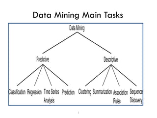
  • 8. DM Task: Descriptive Modeling 9 3.3 3.4 3.5 3.6 3.7 3.8 3.9 4 3.7 3.8 3.9 4 4.1 4.2 4.3 4.4 Red Blood Cell Volume Red Blood Cell Hemoglobin Concentration EM ITERATION 25 • Goal is to build a “descriptive” model that models the underlying observation – e.g., a model that could simulate the data if needed • Description Methods find human-interpretable patterns that describe and find natural groupings of the data. • Methods used in descriptive modeling are: clustering, summarization, association rule discovery, etc. • Descriptive model identifies patterns or relationship in data – Unlike the predictive model, a descriptive model serves as a way to explore the properties of the data examined, not to predict new properties
  • 9. Example of Descriptive Modeling • goal: learn directed relationships among p variables • techniques: directed (causal) graphs • challenge: distinguishing between correlation and causation – Example: Do yellow fingers cause lung cancer? cancer yellow fingers ? smoking hidden cause: smoking 10
  • 10. Pattern (Association Rule) Discovery • Goal is to discover interesting “local” patterns (sequential patterns) in the data rather than to characterize the data globally – Also called link analysis (uncovers relationships among data) • Given market basket data we might discover that – If customers buy wine and bread then they buy cheese with probability 0.9 • Methods used in pattern discovery include: – Association rules, Sequence discovery, etc. 11
  • 11. Example of Pattern Discovery • Example in retail: Customer transactions to consumer behavior: – People who bought “Da Vinci Code” also bought “The Five People You Meet in Heaven” (www.amazon.com) • Example: football player behavior – If player A is in the game, player B’s scoring rate increases from 25% chance per game to 95% chance per game • What about the following? 12 ADACABDABAABBDDBCADDDDBCDDBCCBBCCDADADAADABDBBDABABBCDDDCDDABDC BBDBDBCBBABBBCBBABCBBACBBDBAACCADDADBDBBCBBCCBBBDCABDDBBADDBBBBCC ACDABBABDDCDDBBABDBDDBDDBCACDBBCCBBACDCADCBACCADCCCACCDDADCBCAD ADBAACCDDDCBDBDCCCCACACACCDABDDBCADADBCBDDADABCCABDAACABCABACB DDDCBADCBDADDDDCDDCADCCBBADABBAAADAAABCCBCABDBAADCBCDACBCABABC CBACBDABDDDADAABADCDCCDBBCDBDADDCCBBCDBAADADBCAAAADBDCADBDBBBC DCCBCCCDCCADAADACABDABAABBDDBCADDDDBCDDBCCBBCCDADADACCCDABAABBC BDBDBADBBBBCDADABABBDACDCDDDBBCDBBCBBCCDABCADDADBACBBBCCDBAAADDD BDDCABACBCADCDCBAAADCADDADAABBACCBB
  • 12. 13 Supervised vs. Unsupervised Learning • Supervised learning (classification) – Supervision: The training data (observations, measurements, etc.) are accompanied by labels indicating the class of the observations – New data is classified based on the training set • Unsupervised learning (clustering) – The class labels of training data is unknown – Given a set of measurements, observations, etc. with the aim of establishing the existence of classes or clusters in the data
  • 13. Basic Data Mining algorithms • Classification (which is also called Supervised learning) maps data into predefined groups or classes to enhance the prediction process • Clustering (which is also called Unsupervised learning ) groups similar data together into clusters. – is used to find appropriate groupings of elements for a set of data. – Unlike classification, clustering is a kind of undirected knowledge discovery or unsupervised learning; that is, there is no target field, and the relationship among the data is identified by bottom-up approach. • Association Rule (is also known as market basket analysis) – It discovers interesting associations between attributes contained in a database. – Based on frequency counts of the number of items occur in the event, association rule tells if item X is a part of the event, then what is the percentage of item Y is also part of the event. 14
  • 15. Classification: Definition • Classification is a data mining (machine learning) technique used to predict group membership for data instances. • Given a collection of records (training set), each record contains a set of attributes, one of the attributes is the class. – Find a model for class attribute as a function of the values of other attributes. • Goal: previously unseen records should be assigned a class as accurately as possible. A test set is used to determine the accuracy of the model. – Usually, the given data set is divided into training and test sets, with training set used to build the model and test set used to validate it. • For example, one may use classification to predict whether the weather on a particular day will be “sunny”, “rainy” or “cloudy”. 16
  • 16. 17 Classification—A Two-Step Process • Model construction: describing a set of predetermined classes – Each tuple/sample is assumed to belong to a predefined class, as determined by the class label attribute – The set of tuples used for model construction is training set – The model is represented as classification rules, decision trees, or mathematical formula • Model usage: for classifying future or unknown objects – Estimate accuracy of the model • The known label of test sample is compared with the classified result from the model • Accuracy rate is the percentage of test set samples that are correctly classified by the model • Test set is independent of training set – If the accuracy is acceptable, use the model to classify data tuples whose class labels are not known
  • 17. Illustrating Classification Task Apply Model Induction Deduction Learn Model Model Tid Attrib1 Attrib2 Attrib3 Class 1 Yes Large 125K No 2 No Medium 100K No 3 No Small 70K No 4 Yes Medium 120K No 5 No Large 95K Yes 6 No Medium 60K No 7 Yes Large 220K No 8 No Small 85K Yes 9 No Medium 75K No 10 No Small 90K Yes 10 Tid Attrib1 Attrib2 Attrib3 Class 11 No Small 55K ? 12 Yes Medium 80K ? 13 Yes Large 110K ? 14 No Small 95K ? 15 No Large 67K ? 10 Test Set Learning algorithm Training Set
  • 18. Confusion Matrix for Performance Evaluation • Most widely-used metric is measuring Accuracy of the system : • Other metric for performance evaluation are Precision, Recall & F-Measure PREDICTED CLASS ACTUAL CLASS Class=Yes Class=No Class=Yes a (TP) b (FP) Class=No c (FP) d (TP) 100 * Accuracy FP TP TP d c b a d a + = + + + + =
  • 19. Classification methods • Goal: Predict class Ci = f(x1, x2, .. xn) • There are various classification methods. Popular classification techniques include the following. – K-nearest neighbor – Decision tree classifier: divide decision space into piecewise constant regions. – Neural networks: partition by non-linear boundaries – Bayesian network: a probabilistic model – Support Vector Machine (SVM) 20
  • 20. K-Nearest Neighbors • K-nearest neighbor is a supervised learning algorithm where the result of new instance query is classified based on majority of K-nearest neighbor category. • The purpose of this algorithm is to classify a new object based on attributes and training samples: (xn, f(xn)), n=1..N. • Given a query point, we find K number of objects or (training points) closest to the query point. – The classification is using majority vote among the classification of the K objects. – K Nearest neighbor algorithm used neighborhood classification as the prediction value of the new query instance. • K nearest neighbor algorithm is very simple. It works based on minimum distance from the query instance to the training samples to determine the K-nearest neighbors. 21
  • 21. How to compute K-Nearest Neighbor (KNN) Algorithm? • Determine parameter K = number of nearest neighbors • Calculate the distance between the query-instance and all the training samples – We can use Euclidean distance • Sort the distance and determine nearest neighbors based on the Kth minimum distance • Gather the category of the nearest neighbors • Use simple majority of the category of nearest neighbors as the prediction value of the query instance – Any ties can be broken at random.
  • 22. 23 K Nearest Neighbors: Key issues The key issues involved in training KNN model includes • Setting the variable K - Number of nearest neighbors –The numbers of nearest neighbors (K) should be based on cross validation over a number of K setting. –When k=1 is a good baseline model to benchmark against. –A good rule-of-thumb is that K should be less than or equal to the square root of the total number of training patterns. • Setting the type of distant metric –We need a measure of distance in order to know who are the neighbours –Assume that we have T attributes for the learning problem. Then one example point x has elements xt  , t=1,…T. –The distance between two points xi xj is often defined as the Euclidean distance: 2 1 ) ( ) , (  = − = D i Yi Xi Y X Dist N K 
  • 23. k-Nearest Neighbors (k-NN) ▪ K-NN is an algorithm that can be used when you have a bunch of objects that have been classified or labeled in some way, and other similar objects that haven’t gotten classified or labeled yet, and you want a way to automatically label them ▪ The objects could be data scientists who have been classified as “active” or “passive”; or people who have been labeled as “high credit” or “low credit”; or restaurants that have been labeled “five star,” “four star,” “three star,” “two star,” “one star,” or if they really suck, “zero stars.” ▪ More seriously, it could be patients who have been classified as “high cancer risk” or “low cancer risk.” 24
  • 25. • K-NN is a Supervised machine learning while K- NN is a classification or regression machine learning algorithm • K-NN is a lazy learner while K-Means is an eager learner. An eager learner has a model fitting that means a training step but a lazy learner does not have a training phase. • K-NN performs much better if all of the data have the same scale (Labelled Data) but this is not true for K-means. 26 K-Nearest Neighbor(K-NN)
  • 26. K-Nearest Neighbor Classification (KNN) • Example with credit scores: • Say you have the age, income, and a credit category of high or low for a bunch of people and you want to use the age and income to predict the credit label of “high” or “low” for a new person. • For example, here are the first few rows of a dataset, with income represented in thousands 27
  • 27. K-Nearest Neighbor Classification (KNN) • What if a new guy comes in who is 57 years old and who makes $37,000? What’s his likely credit rating label? 28
  • 29. Hamming Distance • For category variables, Hamming distance can be used. 30
  • 31. What is the most possible label for C? c 32 Solution: Looking for the nearest K neighbors of C. Take the majority label as C’s label Let’s suppose K = 3:
  • 32. What is the most possible label for C? C 33 • The 3 nearest points to C are: a, a and o. • Therefore, the most possible label for C is a.
  • 33. Example • We have data from the questionnaires survey (to ask people opinion) and objective testing with two attributes (acid durability and strength) to classify whether a special paper tissue is good or not. Here is four training samples. • Now the factory produces a new paper tissue that pass laboratory test with X1 = 3 and X2 = 7. – Without undertaking another expensive survey, guess the goodness of the new tissue? – Use squared Euclidean distance for similarity measurement. X1 = Acid Durability (seconds) X2 = Strength (kg/m2) Y = Classification 7 7 Bad 7 4 Bad 3 4 Good 1 4 Good
  • 34. Solution X1 = Acid Durability (seconds) X2 = Strength (kg/m2) Square Distance to query instance (3, 7) Rank minimum distance Is it included in 3- NNs? Y = Category of NN 7 7 3 Yes Bad 7 4 4 No - 3 4 1 Yes Good 1 4 2 Yes Good • Use simple majority of the category of nearest neighbors as the prediction value of the query instance. We have 2 good and 1 bad, since 2>1 then we conclude that a new paper tissue that pass laboratory test with X1 = 3 and X2 = 7 is included in Good category.
  • 35. 37 KNNs: advantages & Disadvantages • Advantage – Nonparametric architecture – Simple – Powerful – Requires no training time • Disadvantage: Difficulties with k-nearest neighbour algorithms – Memory intensive: just store the training examples • when a test example is given then find the closest matches – Classification/estimation is slow – Have to calculate the distance of the test case from all training cases – There may be irrelevant attributes amongst the attributes – curse of dimensionality
  • 37. Decision Trees • Decision tree constructs a tree where internal nodes are simple decision rules on one or more attributes and leaf nodes are predicted class labels. ✓Given an instance of an object or situation, which is specified by a set of properties, the tree returns a "yes" or "no" decision about that instance. Attribute_1 Attribute_2 Attribute_2 value-1 value-2 value-3 Class1 Class1 Class2 Class2 Class1 value-5 value-4 value-6 value-7
  • 38. Choosing the Splitting Attribute • At each node, the best attribute is selected for splitting the training examples using a Goodness function – The best attribute is the one that separate the classes of the training examples faster such that it results in the smallest tree • Typical goodness functions: – information gain, information gain ratio, and Gini index •Information Gain –Select the attribute with the highest information gain, that create small average disorder • First, compute the disorder using Entropy; the expected information needed to classify objects into classes • Second, measure the Information Gain; to calculate by how much the disorder of a set would reduce by knowing the value of a particular attribute.
  • 39. Entropy ) ( log log ) , ( 2 2 S Entropy n n n n n n n n n n D = − − = − − + + − + • The Entropy measures the disorder of a set S containing a total of n examples of which n+ are positive and n- are negative and it is given by: • Some useful properties of the Entropy: – D(n,m) = D(m,n) – D(0,m) = D(m,0) = 0 ✓D(S)=0 means that all the examples in S have the same class – D(m,m) = 1 ✓D(S)=1 means that half the examples in S are of one class and half are in the opposite class
  • 40. Information Gain • The Information Gain measures the expected reduction in entropy due to splitting on an attribute A Parent Node, S is split into k partitions; ni is number of records in partition i • Information Gain: Measures Reduction in Entropy achieved because of the split. Choose the split that achieves most reduction (maximizes GAIN)       − =  = k i i split i Entropy n n S Entropy GAIN 1 ) ( ) (
  • 41. Example 1: The problem of “Sunburn” • You want to predict whether another person is likely to get sunburned if he/she is back to the beach. How can you do this? • Data Collected: predict based on the observed properties of the people Name Hair Height Weight Lotion Result Sarah Blonde Average Light No Sunburned Dana Blonde Tall Average Yes None Alex Brown Short Average Yes None Annie Blonde Short Average No Sunburned Emily Red Average Heavy No Sunburned Pete Brown Tall Heavy No None John Brown Average Heavy No None Kate Blonde Short Light Yes None
  • 42. Attribute Selection by Information Gain to construct the optimal decision tree 954 . 0 8 5 log 8 5 8 3 log 8 3 ) 5 , 3 ( 2 2 = − − = = − + D D({ “Sarah”,“Dana”,“Alex”,“Annie”, “Emily”,“Pete”,“John”,“Katie”}) • Entropy: The Disorder of Sunburned
  • 43. Which decision variable minimises the disorder? Test Average Disorder of the other attributes Hair 0.50 height 0.69 weight 0.94 lotion 0.61 • Which decision variable maximises the Info Gain then? • Remember it’s the one which minimises the average disorder. ✓ Gain(hair) = 0.954 - 0.50 = 0.454 ✓ Gain(height) = 0.954 - 0.69 =0.264 ✓ Gain(weight) = 0.954 - 0.94 =0.014 ✓ Gain (lotion) = 0.954 - 0.61 =0.344
  • 44. The best decision tree? ? is_sunburned Alex Pete John Emily Sunburned = Sarah, Annie, None = Dana, Katie Hair colour brown blonde red • Once we have finished with hair colour we then need to calculate the remaining branches of the decision tree. • Which attributes is better to classify the remaining ?
  • 45. The best Decision Tree Sarah, Annie is_sunburned Alex, Pete, John Emily Dana, Katie Hair colour Lotion used blonde red brown no yes • This is the simplest and optimal one possible and it makes a lot of sense. • It classifies 4 of the people on just the hair colour alone.
  • 46. Sunburn sufferers are ... • You can view Decision Tree as an IF-THEN_ELSE statement which tells us whether someone will suffer from sunburn. If (Hair-Colour=“red”) then return (sunburned = yes) else if (hair-colour=“blonde” and lotion- used=“No”) then return (sunburned = yes) else return (false)
  • 47. 53 Exercise: Decision Tree for “buy computer or not”. Use the training Dataset given below to construct decision tree age income student credit_rating buys_computer <=30 high no fair no <=30 high no excellent no 31…40 high no fair yes >40 medium no fair yes >40 low yes fair yes >40 low yes excellent no 31…40 low yes excellent yes <=30 medium no fair no <=30 low yes fair yes >40 medium yes fair yes <=30 medium yes excellent yes 31…40 medium no excellent yes 31…40 high yes fair yes >40 medium no excellent no
  • 48. 54 Output: A Decision Tree for “buys_computer” age? overcast student? credit rating? <=30 >40 no yes yes yes 31..40 fair excellent yes no
  • 49. Why decision tree induction in DM? Cons - Cannot handle complicated relationship between features - Simple decision boundaries - Problems with lots of missing data Pros + Reasonable training time + Fast application + Easy to interpret + Easy to implement + Can handle large number of features 56 • Relatively faster learning speed (than other classification methods) • Convertible to simple and easy to understand classification if-then- else rules • Comparable classification accuracy with other methods • Does not require any prior knowledge of data distribution, works well on noisy data.
  • 51. Why Bayesian Classification? • Provides practical learning algorithms – Probabilistic learning: Calculate explicit probabilities for hypothesis. E.g. Naïve Bayes • Prior knowledge and observed data can be combined – Incremental: Each training example can incrementally increase/decrease the probability that a hypothesis is correct. • It is a generative (model based) approach, which offers a useful conceptual framework – Probabilistic prediction: Predict multiple hypotheses, weighted by their probabilities. E.g. sequences could also be classified, based on a probabilistic model specification – Any kind of objects can be classified, based on a probabilistic model specification
  • 52. CONDITIONAL PROBABILITY • Probability : How likely is it that an event will happen? • Sample Space S – An event A and C are a subset of S • P(C / A)- Probability that event C occurs given that event A has already occurred. Example of conditional probability: • There are 2 baskets. B1 has 2 red ball and 5 blue ball. B2 has 4 red ball and 3 blue ball. – Find probability of picking a red ball from basket 1? P(red ball | basket 1) = – What about P(basket2 | red ball) ? ) ( ) , ( ) | ( A P C A P A C P =
  • 53. Bayes Classifier • A probabilistic framework for solving classification problems • Bayes theorem: • Example of Bayes Theorem – Given: A doctor knows that meningitis causes stiff neck 50% of the time. Prior probability of any patient having meningitis is 1/50. Prior probability of any patient having stiff neck is 1/20. If a patient has stiff neck, what’s the probability he/she has meningitis? ) ( ) ( ) | ( ) | ( A P C P C A P A C P = ) ( ) , ( ) | ( C P C A P C A P = ) ( ) , ( ) | ( A P C A P A C P =
  • 54. Bayes Theorem • Example 2: A medical cancer diagnosis problem. There are 2 possible outcomes of a diagnosis: +ve, -ve. We know 0.8% of world population has cancer. Test gives correct +ve result 98% of the time and gives correct –ve result 97% of the time. If a patient’s test returns +ve, should we diagnose the patient as having cancer? P(cancer) = 0.008 p(no-cancer) = 0.992 P(+ve|cancer) = 0.98 P(-ve|cancer) = 0.02 P(+ve|no-cancer) = 0.03 P(-ve|no-cancer) = 0.97 Using Bayes Formula: – P(cancer|+ve) = P(+ve|cancer)xP(cancer) / P(+ve) = 0.98 x 0.008 = 0.0078 / P(+ve) – P(no-cancer|+ve) = P(+ve|no-cancer)xP(no-cancer) / P(+ve) = 0.03 x 0.992 = 0.0298 / P(+ve) So, the patient most likely does not have cancer.
  • 55. General Bayes Theorem • Consider each attribute and class label as random variables • Given a record with attributes (A1, A2,…,An) – Goal is to predict class C – Specifically, we want to find the value of C that maximizes P(C| A1, A2,…,An ) • Can we estimate P(C| A1, A2,…,An ) directly from data? – Approach: compute the posterior probability P(C | A1, A2, …, An) for all values of C using the Bayes theorem – Choose value of C that maximizes: P(C | A1, A2, …, An) – Equivalent to choosing value of C that maximizes P(A1, A2, …, An|C) P(C) • How to estimate P(A1, A2, …, An | C )? ) ( ) ( ) | ( ) | ( 2 1 2 1 2 1 n n n A A A P C P C A A A P A A A C P    =
  • 56. Naïve Bayes Classifier • Assume independence among attributes Ai when class is given: – P(A1, A2, …, An |C) = P(A1| Cj) P(A2| Cj)… P(An| Cj) – Can estimate P(Ai| Cj) for all Ai and Cj. – New point is classified to Cj if P(Cj)  P(Ai| Cj) is maximal.  = i j i j j Bayes Naive C A P C P C ) | ( ) ( max arg
  • 57. Example. ‘Play Tennis’ data Day Outlook Temperature Humidity Wind Play Tennis Day1 Sunny Hot High Weak No Day2 Sunny Hot High Strong No Day3 Overcast Hot High Weak Yes Day4 Rain Mild High Weak Yes Day5 Rain Cool Normal Weak Yes Day6 Rain Cool Normal Strong No Day7 Overcast Cool Normal Strong Yes Day8 Sunny Mild High Weak No Day9 Sunny Cool Normal Weak Yes Day10 Rain Mild Normal Weak Yes Day11 Sunny Mild Normal Strong Yes Day12 Overcast Mild High Strong Yes Day13 Overcast Hot Normal Weak Yes Day14 Rain Mild High Strong No • Suppose that you have a free afternoon and you are thinking whether or not to go and play tennis, How you do that? ✓Based on the following training data, predict when this player will Play Tennis?
  • 58. Naive Bayes Classifier • Given a training set, we can compute the probabilities Outlook P N Humidity P N sunny 2/9 3/5 high 3/9 4/5 overcast 4/9 0 normal 6/9 1/5 rain 3/9 2/5 Tempreature Windy hot 2/9 2/5 Strong 3/9 3/5 mild 4/9 2/5 Weak 6/9 2/5 cool 3/9 1/5 P(P) = 9/14 P(N) = 5/14 Where, P(P) is the probability of playing tennis = Yes and P(n) is the probability of playing tennis = No
  • 59. • Based on the model created, predict Play Tennis or Not for the following unseen sample (Outlook=Sunny, Temperature=Cool, Humidity=High, Wind=Strong) • Working: ) | ( ) | ( ) | ( ) | ( ) ( max arg ) | ( ) ( max arg ] , [ ] , [ C strong Wind P C high Hum P C cool Temp P C sunny Outl P C P C a P C P C no yes C t t no yes C NB = = = = = =    no PlayTennis answer no strong P no high P no cool P no sunny P no P yes strong P yes high P yes cool P yes sunny P yes P =  = = : ) | ( ) | ( ) | ( ) | ( ) ( 0053 . 0 ) | ( ) | ( ) | ( ) | ( ) ( 0.0206 Play-tennis example • More example: What if the following test data is given: X= <Outlook=rain, Temperature=hot, Humidity=high, Wind=weak>
  • 60. Exercise: Naïve Bayes Classifier Name Give Birth Can Fly Live in Water Have Legs Class human yes no no yes mammals python no no no no non-mammals salmon no no yes no non-mammals whale yes no yes no mammals frog no no sometimes yes non-mammals komodo no no no yes non-mammals bat yes yes no yes mammals pigeon no yes no yes non-mammals cat yes no no yes mammals leopard shark yes no yes no non-mammals turtle no no sometimes yes non-mammals penguin no no sometimes yes non-mammals porcupine yes no no yes mammals eel no no yes no non-mammals salamander no no sometimes yes non-mammals gila monster no no no yes non-mammals platypus no no no yes mammals owl no yes no yes non-mammals dolphin yes no yes no mammals eagle no yes no yes non-mammals Give Birth Can Fly Live in Water Have Legs Class yes no yes no ? 0027 . 0 20 13 004 . 0 ) ( ) | ( 021 . 0 20 7 06 . 0 ) ( ) | ( 0042 . 0 13 4 13 3 13 10 13 1 ) | ( 06 . 0 7 2 7 2 7 6 7 6 ) | ( =  = =  = =    = =    = N P N A P M P M A P N A P M A P A: attributes M: mammals N: non-mammals P(A|M)P(M) > P(A|N)P(N) => Mammals
  • 62. 71 Brain vs. Machine • The Brain – Pattern Recognition – Association – Complexity – Noise Tolerance • The Machine – Calculation – Precision – Logic
  • 63. 72 Features of the Brain • Ten billion (1010) neurons ✓ Neuron switching time >10-3secs • Face Recognition ~0.1secs • On average, each neuron has several thousand connections • Hundreds of operations per second • High degree of parallel computation • Distributed representations • Die off frequently (never replaced) • Compensated for problems by massive parallelism
  • 64. Neural Network • Computing systems modeled after the brain’s networks of interconnected processing elements (neurons) • Interconnected processors operate in parallel and interact with each other • Allows the network to learn from the data it processes • capable of finding and differentiating
  • 65. • Neural Networks can: • Learn and adjust to new circumstances on their own • Take part in massive parallel processing • Function without complete information • Cope with huge volumes of information • Analyze nonlinear relationships Chapter II – Organization & IS
  • 66. Neural Network classifier • It is represented as a layered set of interconnected processors. These processor nodes has a relationship with the neurons of the brain. Each node has a weighted connection to several other nodes in adjacent layers. Individual nodes take the input received from connected nodes and use the weights together to compute output values. • The inputs are fed simultaneously into the input layer. • The weighted outputs of these units are fed into hidden layer. • The weighted outputs of the last hidden layer are inputs to units making up the output layer. 75
  • 67. Architecture of Neural network • Neural networks are used to look for patterns in data, learn these patterns, and then classify new patterns & make forecasts • A network with the input and output layer only is called single- layered neural network. Whereas, a multilayer neural network is a generalized one with one or more hidden layer. – A network containing two hidden layers is called a three-layer neural network, and so on. Hidden nodes Output nodes x1 x2 x3 x1 x2 x3 w1 w2 w3 y n i i i e y x w o − = + = =  1 1 ) ( ) ( 1   Single layered NN Multilayer NN Input nodes
  • 68. A Multilayer Neural Network • INPUT: records with class attribute with normalized attributes values. –INPUT VECTOR: X = { x1, x2, …. xm}, where m is the number of attributes. –INPUT LAYER – there are as many nodes as class attributes i.e. as the length of the input vector. • HIDDEN LAYER – neither its input nor its output can be observed from outside. –The number of nodes in the hidden layer and the number of hidden layers depends on implementation. Input layer Hidden layer Output layer • OUTPUT LAYER – corresponds to the class attribute. –There are as many nodes as classes (values of the class attribute). –Ok, where k= 1, 2,.. n, where n is number of classes
  • 69. Hidden layer: Neuron with Activation • The neuron is the basic information processing unit of a NN. It consists of: 1 A set of links, describing the neuron inputs, with weights W1, W2, …, Wm 2. An adder function (linear combiner) for computing the weighted sum of the inputs (real numbers): 3. Activation function (also called squashing function): for limiting the output behavior of the neuron.  = = m 1 j jx w y j ) (y y b + =
  • 70. Activation Functions •(a) is a step function or threshold function (hardlimiting): •(b) is a sigmoid function: 1/(1+e-x) •Changing the bias weight W0,i moves the threshold location –Bias helps the neural network to be more flexible since it adjust the activation function left-or-right, making it centered on some other value than x = 0. To this effect an additional node is added to the input layer, with its constant input; say, 1 or -1, … When this is multiplied by the weights of the hidden layer, it provides a bias (DC offset) to activation function.
  • 71. Two Topologies of neural network • NN can be designed in a feed forward or recurrent manner • In a feed forward neural network connections between the units do not form a directed cycle. – In this network, the information moves in only one direction, forward, from the input nodes, through the hidden nodes (if any) & to the output nodes. There are no cycles or loops or no feedback connections are present in the network, that is, connections extending from outputs of units to inputs of units in the same layer or previous layers. • In recurrent networks data circulates back & forth until the activation of the units is stabilized – Recurrent networks have a feedback loop where data can be fed back into the input at some point before it is fed forward again for further processing and final output. 81
  • 72. Training the neural network • The purpose is to learn to generalize using a set of sample patterns where the desired output is known. • Back Propagation is the most commonly used method for training multilayer feed forward NN. – Back propagation learns by iteratively processing a set of training data (samples). – For each sample, weights are modified to minimize the error between the desired output and the actual output. • After propagating an input through the network, the error is calculated and the error is propagated back through the network while the weights are adjusted in order to make the error smaller. 82
  • 73. Training Algorithm •The applied learning algorithm is as follows –Initialize the weights and threshold to small random numbers. –Present a vector x to the neuron inputs and calculate the output using the adder function. –Apply the activation function such that –Update the weights according to the error. j T j j x y y W W * ) ( * − + =   = = m 1 j jx w y j        = 0 y if 1 0 y if 0 y
  • 74. ANN Training Example • Training – epoch 1: y1 = 0.92*0 + 0.62*0 – 0.22 = -0.22 → y = 0 y2 = 0.92*1 + 0.62*0 – 0.22 = 0.7 → y =1 W1(1) = 0.92 + 0.1 * (0 – 1) * 1 = 0.82 W2(1) = 0.62 + 0.1 * (0 – 1) * 0 = 0.62 W0(1) = 0.22 + 0.1 * (0 – 1) * (-1)= 0.32 y3 = 0.82*0 + 0.62*1 – 0.32 = 0.3 → y = 1 y4 = 0.82*1 + 0.62*1 – 0.32 = 1.12 → y =1 X Bias 1st input (x1) 2nd input (x2) Target output -1 0 0 0 -1 1 0 0 -1 0 1 1 -1 1 1 1 Given the following two inputs x1, x2; find equation that helps to draw the boundary? • Let say we have the following initializations: W1(0) = 0.92, W2(0) = 0.62, W0(0) = 0.22, ή = 0.1
  • 75. ANN Training Example • Training – epoch 2: y1 = 0.82*0 + 0.62*0 – 0.32 = -0.32 → y= 0 y2 = 0.82*1 + 0.62*0 – 0.32 = 0.5 → y= 1 W1(2) = 0.82 + 0.1 * (0 – 1) * 1 = 0.72 W2(2) = 0.62 + 0.1 * (0 – 1) * 0 = 0.62 W0(2) = 0.32 + 0.1 * (0 – 1) * (-1)= 0.42 y3 = 0.72*0 + 0.62*1 – 0.42 = 0.2 → y= 1 y4 = 0.72*1 + 0.62*1 – 0.42 = 0.92 → y = 1 • Training – epoch 3: y1 = 0.72*0 + 0.62*0 – 0.42 = -0.42 → y = 0 y2 = 0.72*1 + 0.62*0 – 0.42 = 0.4 → y = 1 W1(3) = 0.72 + 0.1 * (0 – 1) * 1 = 0.62 W2(3) = 0.62 + 0.1 * (0 – 1) * 0 = 0.62 W0(3) = 0.42 + 0.1 * (0 – 1) * (-1)= 0.52 y3 = 0.62*0 + 0.62*1 – 0.52 = 0.1→ y = 1 y4 = 0.62*1 + 0.62*1 – 0.52 = 0.72→ y = 1 X X
  • 76. ANN Training Example • Training – epoch 4: y1 = 0.62*0 + 0.62*0 – 0.52 = -0.52 → y = 0 y2 = 0.62*1 + 0.62*0 – 0.52 = 0.10→ y = 1 W1(4) = 0.62 + 0.1 * (0 – 1) * 1 = 0.52 W2(4) = 0.62 + 0.1 * (0 – 1) * 0 = 0.62 W0(4) = 0.52 + 0.1 * (0 – 1) * (-1)= 0.62 y3 = 0.52*0 + 0.62*1 – 0.62 = 0 → y = 0 W1(4) = 0.52 + 0.1 * (1 – 0) * 0 = 0.52 W2(4) = 0.62 + 0.1 * (1 – 0) * 1 = 0.72 W0(4) = 0.62 + 0.1 * (1 – 0) * (-1)= 0.52 y4 = 0.52*1 + 0.72*1 – 0.52 = 0.72 → y = 1 • Finally: y1 = 0.52*0 + 0.72*0 – 0.52 = -0.52 → y = 0 y2 = 0.52*1 + 0.72*0 – 0.52 = -0.0 → y = 0 y3 = 0.52*0 + 0.72*1 – 0.52 = 0.2 → y= 1 y4 = 0.52*1 + 0.72*1 – 0.52 = 0.72 → y= 1 X X
  • 77. ANN Training Example + + 1 o 1 0 x2 x1 o + + 1 o 1 0 x2 x1 o
  • 78. Pros and Cons of Neural Network Cons -Slow training time - Hard to interpret & understand the learned function (weights) -Hard to implement: trial & error for choosing number of nodes Pros + Can learn more complicated class boundaries + Fast application + Can handle large number of features Neural Network needs long time for training. Neural Network has a high tolerance to noisy and incomplete data Conclusion: Use neural nets only if decision-trees fail. 91 • Useful for learning complex data like handwriting, speech and image recognition