VV

1. 1
Cluster Analysis
 Cluster: A collection of data objects
 similar (or related) to one another within the same group
 dissimilar (or unrelated) to the objects in other groups
 Cluster analysis (or clustering, data segmentation, …)
 Finding similarities between data according to the
characteristics found in the data and grouping similar
data objects into clusters
 Unsupervised learning: no predefined classes (i.e., learning
by observations vs. learning by examples: supervised

2. 2
Clustering for Data Understanding and
Applications
 Biology: taxonomy of living things: kingdom, phylum, class, order,
family, genus and species
 Information retrieval: document clustering
 Land use: Identification of areas of similar land use in an earth
observation database
 Marketing: Help marketers discover distinct groups in their customer
bases, and then use this knowledge to develop targeted marketing
programs
 City-planning: Identifying groups of houses according to their house
type, value, and geographical location
 Earth-quake studies: Observed earth quake epicenters should be
clustered along continent faults
 Climate: understanding earth climate, find patterns of atmospheric
and ocean
 Economic Science: market resarch

3. 3
Clustering as a Preprocessing Tool (Utility)
 Summarization:
 Preprocessing for regression, PCA, classification, and
association analysis
 Compression:
 Image processing: vector quantization
 Finding K-nearest Neighbors
 Localizing search to one or a small number of clusters
 Outlier detection
 Outliers are often viewed as those “far away” from any
cluster

4. Quality: What Is Good Clustering?
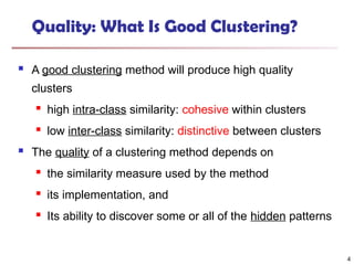
 A good clustering method will produce high quality
clusters
 high intra-class similarity: cohesive within clusters
 low inter-class similarity: distinctive between clusters
 The quality of a clustering method depends on
 the similarity measure used by the method
 its implementation, and
 Its ability to discover some or all of the hidden patterns
4

5. Measure the Quality of Clustering
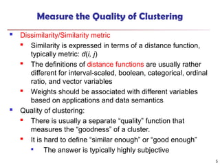
 Dissimilarity/Similarity metric
 Similarity is expressed in terms of a distance function,
typically metric: d(i, j)

The definitions of distance functions are usually rather
different for interval-scaled, boolean, categorical, ordinal
ratio, and vector variables
 Weights should be associated with different variables
based on applications and data semantics
 Quality of clustering:
 There is usually a separate “quality” function that
measures the “goodness” of a cluster.

It is hard to define “similar enough” or “good enough”

The answer is typically highly subjective
5

6. 6

7. Distance measures
7

8. 8
Graphic Representation
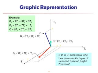
Example:
D1 = 2T1 + 3T2 + 5T3
D2 = 3T1 + 7T2 + T3
Q = 0T1 + 0T2 + 2T3
T3
T1
T2
D1 = 2T1+ 3T2 + 5T3
D2 = 3T1 + 7T2 + T3
Q = 0T1 + 0T2 + 2T3
7
3
2
5
• Is D1 or D2 more similar to Q?
• How to measure the degree of
similarity? Distance? Angle?
Projection?

9. 9
Inner Product -- Examples
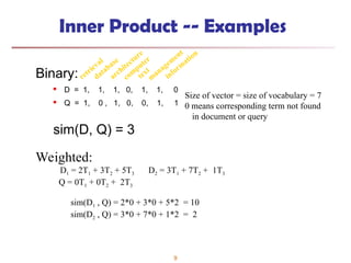
Binary:
 D = 1, 1, 1, 0, 1, 1, 0
 Q = 1, 0 , 1, 0, 0, 1, 1
sim(D, Q) = 3
retrieval
database
architecture
com
puter
text
m
anagem
ent
inform
ation
Size of vector = size of vocabulary = 7
0 means corresponding term not found
in document or query
Weighted:
D1 = 2T1 + 3T2 + 5T3 D2 = 3T1 + 7T2 + 1T3
Q = 0T1 + 0T2 + 2T3
sim(D1 , Q) = 2*0 + 3*0 + 5*2 = 10
sim(D2 , Q) = 3*0 + 7*0 + 1*2 = 2

10. 10
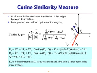
Cosine Similarity Measure
 Cosine similarity measures the cosine of the angle
between two vectors.
 Inner product normalized by the vector lengths.
D1 = 2T1 + 3T2 + 5T3 CosSim(D1 , Q) = 10 / (4+9+25)(0+0+4) = 0.81
D2 = 3T1 + 7T2 + 1T3 CosSim(D2 , Q) = 2 / (9+49+1)(0+0+4) = 0.13
Q = 0T1 + 0T2 + 2T3

t3
t1
t2
D1
D2
Q

D1 is 6 times better than D2 using cosine similarity but only 5 times better using
inner product.
 

 






t
i
t
i
t
i
w
w
w
w
q
d
q
d
iq
ij
iq
ij
j
j
1 1
2
2
1
)
(




CosSim(dj, q) =

11. The K-Means Clustering Method
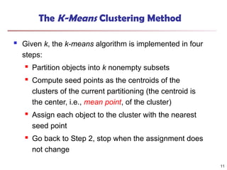
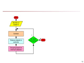
 Given k, the k-means algorithm is implemented in four
steps:
 Partition objects into k nonempty subsets
 Compute seed points as the centroids of the
clusters of the current partitioning (the centroid is
the center, i.e., mean point, of the cluster)
 Assign each object to the cluster with the nearest
seed point
 Go back to Step 2, stop when the assignment does
not change
11

12. 12

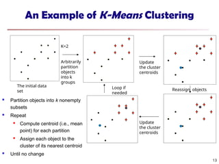
13. An Example of K-Means Clustering
K=2
Arbitrarily
partition
objects
into k
groups
Update
the cluster
centroids
Update
the cluster
centroids
Reassign objects
Loop if
needed
13
The initial data
set
 Partition objects into k nonempty
subsets
 Repeat

Compute centroid (i.e., mean
point) for each partition
 Assign each object to the
cluster of its nearest centroid
 Until no change

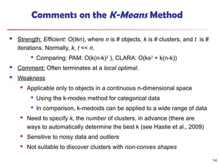
14. Comments on the K-Means Method
 Strength: Efficient: O(tkn), where n is # objects, k is # clusters, and t is #
iterations. Normally, k, t << n.

Comparing: PAM: O(k(n-k)2
), CLARA: O(ks2
+ k(n-k))
 Comment: Often terminates at a local optimal.
 Weakness

Applicable only to objects in a continuous n-dimensional space

Using the k-modes method for categorical data

In comparison, k-medoids can be applied to a wide range of data

Need to specify k, the number of clusters, in advance (there are
ways to automatically determine the best k (see Hastie et al., 2009)
 Sensitive to noisy data and outliers
 Not suitable to discover clusters with non-convex shapes
14

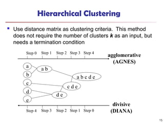
15. Hierarchical Clustering
 Use distance matrix as clustering criteria. This method
does not require the number of clusters k as an input, but
needs a termination condition
Step 0 Step 1 Step 2 Step 3 Step 4
b
d
c
e
a
a b
d e
c d e
a b c d e
Step 4 Step 3 Step 2 Step 1 Step 0
agglomerative
(AGNES)
divisive
(DIANA)
15

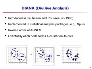
16. DIANA (Divisive Analysis)
 Introduced in Kaufmann and Rousseeuw (1990)
 Implemented in statistical analysis packages, e.g., Splus
 Inverse order of AGNES
 Eventually each node forms a cluster on its own
0
1
2
3
4
5
6
7
8
9
10
0 1 2 3 4 5 6 7 8 9 10
0
1
2
3
4
5
6
7
8
9
10
0 1 2 3 4 5 6 7 8 9 10
0
1
2
3
4
5
6
7
8
9
10
0 1 2 3 4 5 6 7 8 9 10
16

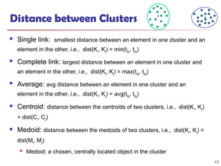
17. Distance between Clusters
 Single link: smallest distance between an element in one cluster and an
element in the other, i.e., dist(Ki, Kj) = min(tip, tjq)
 Complete link: largest distance between an element in one cluster and
an element in the other, i.e., dist(Ki, Kj) = max(tip, tjq)
 Average: avg distance between an element in one cluster and an
element in the other, i.e., dist(Ki, Kj) = avg(tip, tjq)
 Centroid: distance between the centroids of two clusters, i.e., dist(Ki, Kj)
= dist(Ci, Cj)
 Medoid: distance between the medoids of two clusters, i.e., dist(Ki, Kj) =
dist(Mi, Mj)
 Medoid: a chosen, centrally located object in the cluster
X X
17

18. Density-Based Clustering Methods
 Clustering based on density (local cluster criterion), such
as density-connected points

Major features:

Discover clusters of arbitrary shape

Handle noise

One scan

Need density parameters as termination condition
 :
 DBSCAN: Ester, et al. (KDD’96)
18

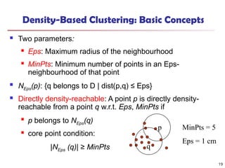
19. Density-Based Clustering: Basic Concepts
 Two parameters:
 Eps: Maximum radius of the neighbourhood
 MinPts: Minimum number of points in an Eps-
neighbourhood of that point
 NEps(p): {q belongs to D | dist(p,q) ≤ Eps}
 Directly density-reachable: A point p is directly density-
reachable from a point q w.r.t. Eps, MinPts if

p belongs to NEps(q)
 core point condition:
|NEps (q)| ≥ MinPts
MinPts = 5
Eps = 1 cm
p
q
19

20. Density-Reachable and Density-Connected
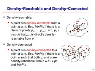
 Density-reachable:

A point p is density-reachable from a
point q w.r.t. Eps, MinPts if there is a
chain of points p1, …, pn, p1 = q, pn =
p such that pi+1 is directly density-
reachable from pi
 Density-connected

A point p is density-connected to a
point q w.r.t. Eps, MinPts if there is a
point o such that both, p and q are
density-reachable from o w.r.t. Eps
and MinPts
p
q
p1
p q
o
20

21. DBSCAN: Density-Based Spatial Clustering of
Applications with Noise
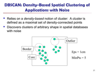
 Relies on a density-based notion of cluster: A cluster is
defined as a maximal set of density-connected points
 Discovers clusters of arbitrary shape in spatial databases
with noise
Core
Border
Outlier
Eps = 1cm
MinPts = 5
21

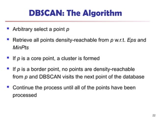
22. DBSCAN: The Algorithm
 Arbitrary select a point p
 Retrieve all points density-reachable from p w.r.t. Eps and
MinPts
 If p is a core point, a cluster is formed
 If p is a border point, no points are density-reachable
from p and DBSCAN visits the next point of the database
 Continue the process until all of the points have been
processed
22

23. DBSCAN: Sensitive to Parameters
23