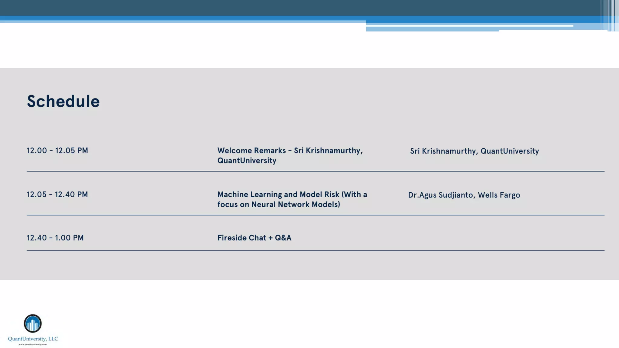
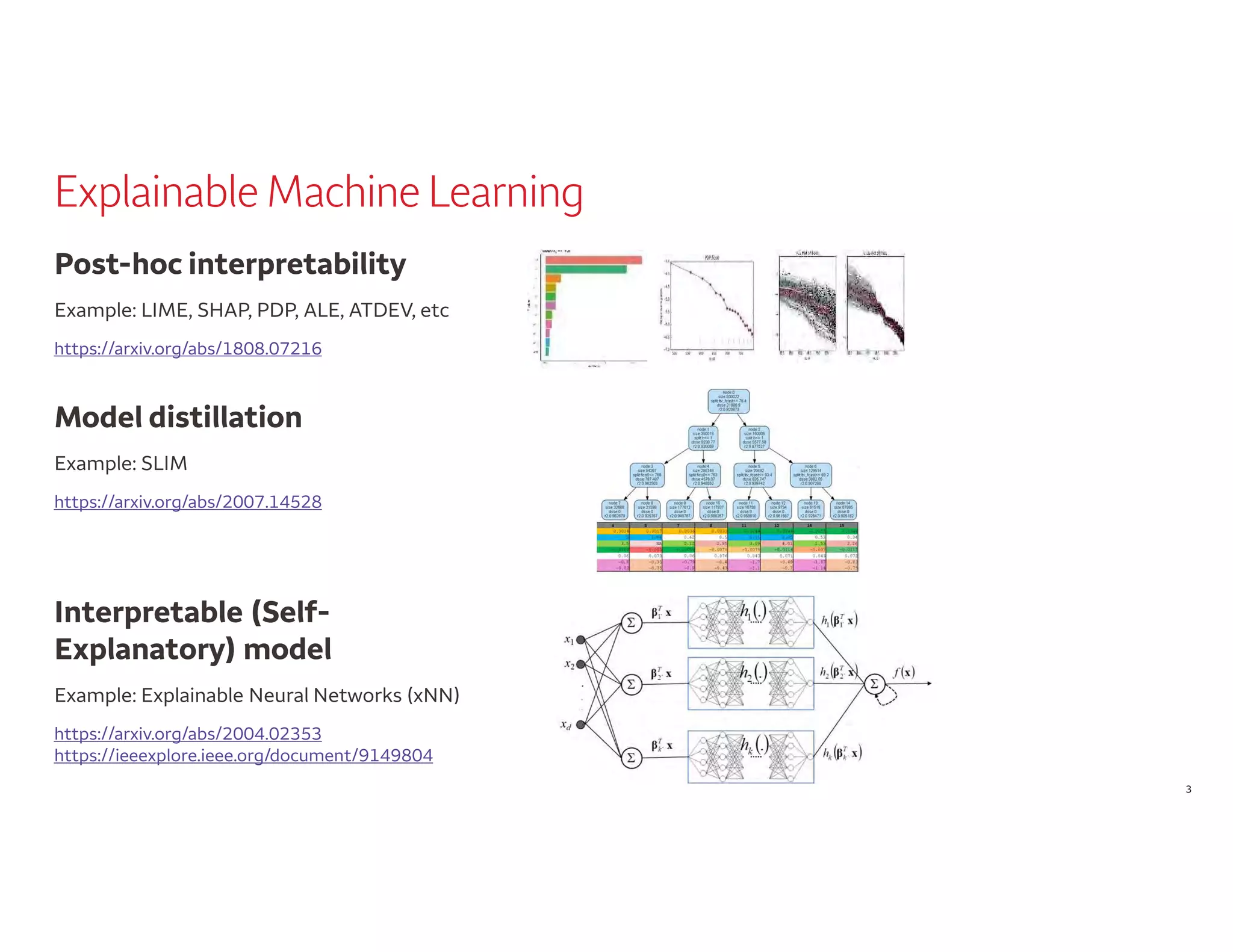
The document outlines a presentation by Dr. Agus Sudjianto on machine learning and model risk, focusing on self-explanatory models and their interpretability. It details his background in model risk management at Wells Fargo and previous roles at Lloyds Banking Group and Bank of America. The presentation emphasizes techniques like local linear models for interpretability and diagnostics in deep neural networks, alongside providing insights into model simplification methods.

1. Qu Speaker Series
Machine Learning and Model Risk
Self-Explanatory Models: Interpretability, Diagnostics and Simplification
Dr. Agus Sudjianto
Wells Fargo
2020 Copyright QuantUniversity LLC.
Hosted By:
Sri Krishnamurthy, CFA, CAP
sri@quantuniversity.com
www.qu.academy
12/09/2020
Online
https://quspeakerseries17.spl
ashthat.com/

2. 2
QuantUniversity
• Boston-based Data Science, Quant
Finance and Machine Learning
training and consulting advisory
• Trained more than 1000 students in
Quantitative methods, Data Science
and Big Data Technologies using
MATLAB, Python and R
• Building a platform for AI
and Machine Learning Exploration
and Experimentation

3. 3
For registration information, go to
https://QuFallSchool.splashthat.com

4. 4
https://Quwinterschool.splashthat.com

5. 5
Next Week

6. 6

7. 7
• Dr.Agus Sudjianto is an executive vice president and head of Corporate Model Risk
for Wells Fargo, where he is responsible for enterprise model risk management.
• Prior to his current position, Agus was the modeling and analytics director and chief
model risk officer at Lloyds Banking Group in the United Kingdom. Before joining
Lloyds, he was a senior credit risk executive and head of Quantitative Risk at Bank
of America.
• Agus holds several U.S. patents in both finance and engineering. He has published
numerous technical papers and is a co-author of Design and Modeling for
Computer Experiments. His technical expertise and interests include quantitative
risk, particularly credit risk modeling, machine learning and computational
statistics.
• Agus holds masters and doctorate degrees in engineering and management from
Wayne State University and the Massachusetts Institute of Technology.
Machine Learning and Model Risk

9. © 2020 Wells Fargo Bank, N.A. All rights reserved. Public.
ReLU DNN as Self-Explanatory Models:
Interpretability, Diagnostics and Simplification
Paper: https://arxiv.org/abs/2011.04041
Aletheia© Python Package: https://github.com/SelfExplainML/Aletheia
Agus Sudjianto
EVP, Head of Corporate Model Risk

10. Acknowledgments
Special thanks to the outstanding contributions from
– William Knauth
– Zebin Yang
– Aijun Zhang
– Rahul Singh
– Vivien Zhao
– Soroush Aramideh
2

11. Explainable Machine Learning
Post-hoc interpretability
Example: LIME, SHAP, PDP, ALE, ATDEV, etc
https://arxiv.org/abs/1808.07216
Model distillation
Example: SLIM
https://arxiv.org/abs/2007.14528
Interpretable (Self-
Explanatory) model
Example: Explainable Neural Networks (xNN)
https://arxiv.org/abs/2004.02353
https://ieeexplore.ieee.org/document/9149804
3

12. From Splines to Neural Networks
Linear Model:
Nonlinear f(x) : Splines Nonlinear f(x) : Neural Networks
Bj(.) is ReLU (Rectifier Linear Units), max(0, zj)
4
Single Index Model Single Hidden Layer Network

13. Deep ReLU Network
Each hidden layer:
• Linear: affine transformation
• Nonlinear: ReLU activation
max 0,
Output layer:
! " # $ $
% $
GLM (generalized linear model)
5

14. Activation Pattern and Oblique Data Partition
Each activation pattern corresponds to a convex region partitioning of the input domain.
Activation Pattern: binary vector with entries indicating the on/off state of each
hidden node.
6

15. 7
Equivalent Local Linear Model Representation
Using the binary diagonal matrix induced from the layerwise activation
pattern
we obtain the closed-form local linear representation for deep ReLU
networks.

16. Example of Activation Pattern and LLM
Activation Patterns
• Local linear models
• Sample partitions
x1 + 4 x2 + 2
8

17. Extraction of Local Linear Models
Aletheia© Python Package: https://github.com/SelfExplainML/Aletheia
Small # active activation patterns
• #LLMS << expressivity
• Many LLMs with single sample or single class
9

18. LLM-based Interpretability
• Local Exact Interpretability (vs. LIME/SHAP)
• Boxplot or Parallel Coordinate Plot
• Feature Importance
• Local Linear Profile Plot (partial dependence)
• Matrix Plot for detection of nonlinear main
effect and pairwise interaction effects
• Regionwise Statitical Inference ……
10

19. 11
Local Exact Interpretability
In constrast, LIME generates inexact and inconsistent local interpretation (due to perturbation)
Post-hoc explanations by SHAP (KernelSHAP, DeepSHAP) can be easily provide misinterpretation
Single instance prediction by ReLU DNN can be interpreted exactly and consistently.

20. 12
Feature Importance and Partial Dependence

21. 13
Nonlinearity and Interaction Detection
Matrix plot of LLM weights vs. region
means
• Diagonal plots – checking nonlinearity
• Off-diagonal plots – checking interactions
Example: Boston Housing Dataset
• CRIM: per-capita crime rate by town
• RM: average number of rooms
• TAX: property-tax rate
• LSTAT: % lower status of population

22. LLM Diagnostics
• Understanding the support (sample) size of
each LLMs → small sample maybe unreliable
• Understanding local and not only aggregated
performance
• Identifying duplicate (unnecessary) LLMs
• Exploring potential model simplification by
comparing local and global performance
• Evaluating the network using testing data and
identifying underexposed/undertrained LLMs
14

23. Identifying Problem with DNN: Simple Example
15
Example:
• 3 hidden-layer NN with 10 neurons in
each layer
• AUC on validation set: 0.8345 vs. 0.835
from data
• Total Number of activation patterns:
3426 LLMs
• 2159 out of 3426 configurations
(%63) have only 1 observation
• LLMs coefficients in DNN maybe less
reliable
Coefficients of X6 in all activation patterns (LLMs)

24. 16
LLM-based Simplification: Merging and Flattening
Merging
• Merging neighboring regions with
similar LLMs
• Benefit:
• Ensuring conceptual soundness
• Improving interpretability
• Controlling model failures
Flattening and Pruning
• Represent LLMs as single hidden layer
network
• Benefit:
• Simpler model
• Less computation resource

25. Example: Model Simplification of Home Lending
17
• Simpler model
• Interpretable
• Better performance and more reliableOriginal DNN
Simplified Model
Region Count
Response
Mean
Response
Std
Local AUC
Global
AUC
0 5873 0.514 0.499 0.836 0.845
1 1801 0.379 0.485 0.828 0.832
2 326 0.907 0.289 0.777 0.727
ReLU DNN Merged Flattened
Training AUC 0.879 0.846 0.847
Testing AUC 0.827 0.827 0.832

26. Example: CNN Text Classification Model
https://arxiv.org/abs/2008.11825
18
Observation
• Many partition into positive and negative response
• Global AUC > Local AUC

27. Log10 counts
LLM Results
663 LLM regions
• There are 401 regions that have <=5 sample points.
• There are 197 regions that have only 1 sample
point.
• Most regions has imbalanced samples of Positive
v.s. Negative reviews.
• All coefficients are very similar
19
#samples (log 10 scale)
#regions

28. Response Distributions of Some LLM Regions
#samples
#samples#samples
#samples
Score Score
Score Score

29. Region-wise Analysis Results
Example Region 0: 3857 samples.
• Example n-grams for top 10 weights of top 10 samples.
• Each row stands for a filter out of 150 filters. Ordered by negative
weights.
Sample#

30. 9
Demos, slides and video available on QuAcademy
Go to www.qu.academy
9

31. 10
Instructions for the Lab:
1. Go to https://academy.qusandbox.com/#/register and register using the code:
"QUFALLSCHOOL"

32. Thank you!
Sri Krishnamurthy, CFA, CAP
Founder and CEO
QuantUniversity LLC.
srikrishnamurthy
www.QuantUniversity.com
Contact
Information, data and drawings embodied in this presentation are strictly a property of QuantUniversity LLC. and shall not be
distributed or used in any other publication without the prior written consent of QuantUniversity LLC.
11