3 DM Classification HFCS kilometres .ppt

DM Task: Predictive Modeling
• A predictive model makes a prediction/forecast about
values of data using known results found from different
historical data
– Prediction Methods use existing variables to predict unknown or
future values of other variables.
• Predict one variable Y given a set of other variables X. Here
X could be an n-dimensional vector
– In effect this is function approximation through learning the
relationship between Y and X
• Many, many algorithms for predictive modeling in
statistics and machine learning, including
– Classification, regression, etc.
• Often the emphasis is on predictive accuracy, less
emphasis on understanding the model
2

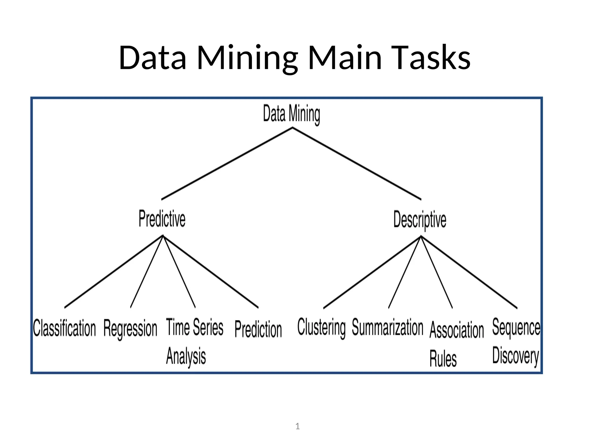
3
• Classification
– predicts categorical class labels (discrete or nominal)
– classifies data (constructs a model) based on the
training set and the values (class labels) in a classifying
attribute and uses it in classifying new data
• Numeric Prediction
– models continuous-valued functions, i.e., predicts
unknown or missing values
Prediction Problems:
Classification vs. Numeric Prediction

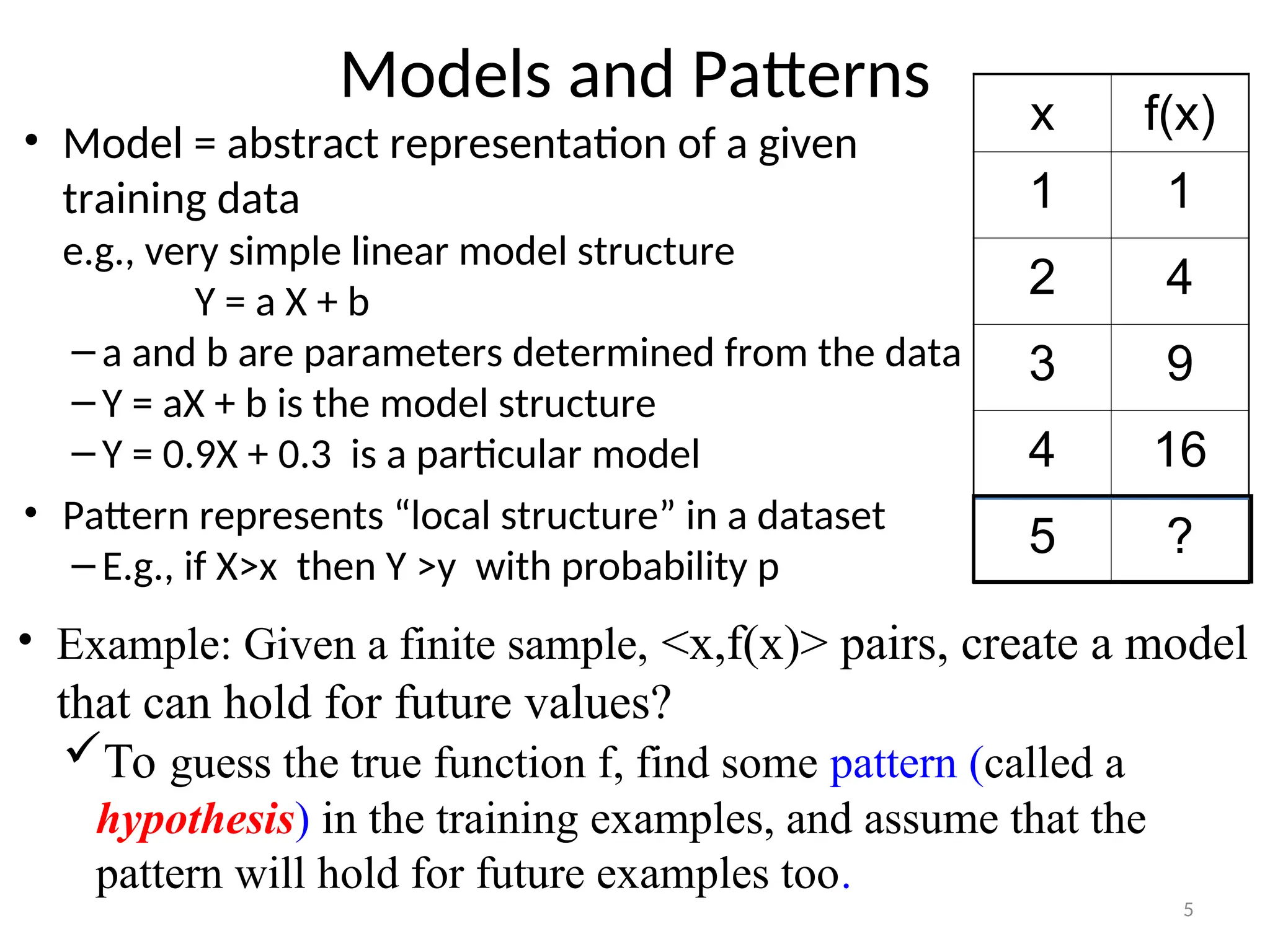
Models and Patterns
• Model = abstract representation of a given
training data
e.g., very simple linear model structure
Y = a X + b
– a and b are parameters determined from the data
– Y = aX + b is the model structure
– Y = 0.9X + 0.3 is a particular model
• Pattern represents “local structure” in a dataset
– E.g., if X>x then Y >y with probability p
5
x f(x)
1 1
2 4
3 9
4 16
5 ?
• Example: Given a finite sample, <x,f(x)> pairs, create a model
that can hold for future values?
To guess the true function f, find some pattern (called a
hypothesis) in the training examples, and assume that the
pattern will hold for future examples too.

Predictive Modeling: Customer Scoring
• Example: a bank has a database of 1 million past
customers, 10% of whom took out mortgages
– Use machine learning to rank new customers as a function of
p(mortgage|customer data)
• Customer data
– History of transactions with the bank
– Other credit data (obtained from Experian, etc)
– Demographic data on the customer or where they live
• Techniques
– Binary classification: logistic regression, decision trees,
etc
– Many, many applications of this nature
6

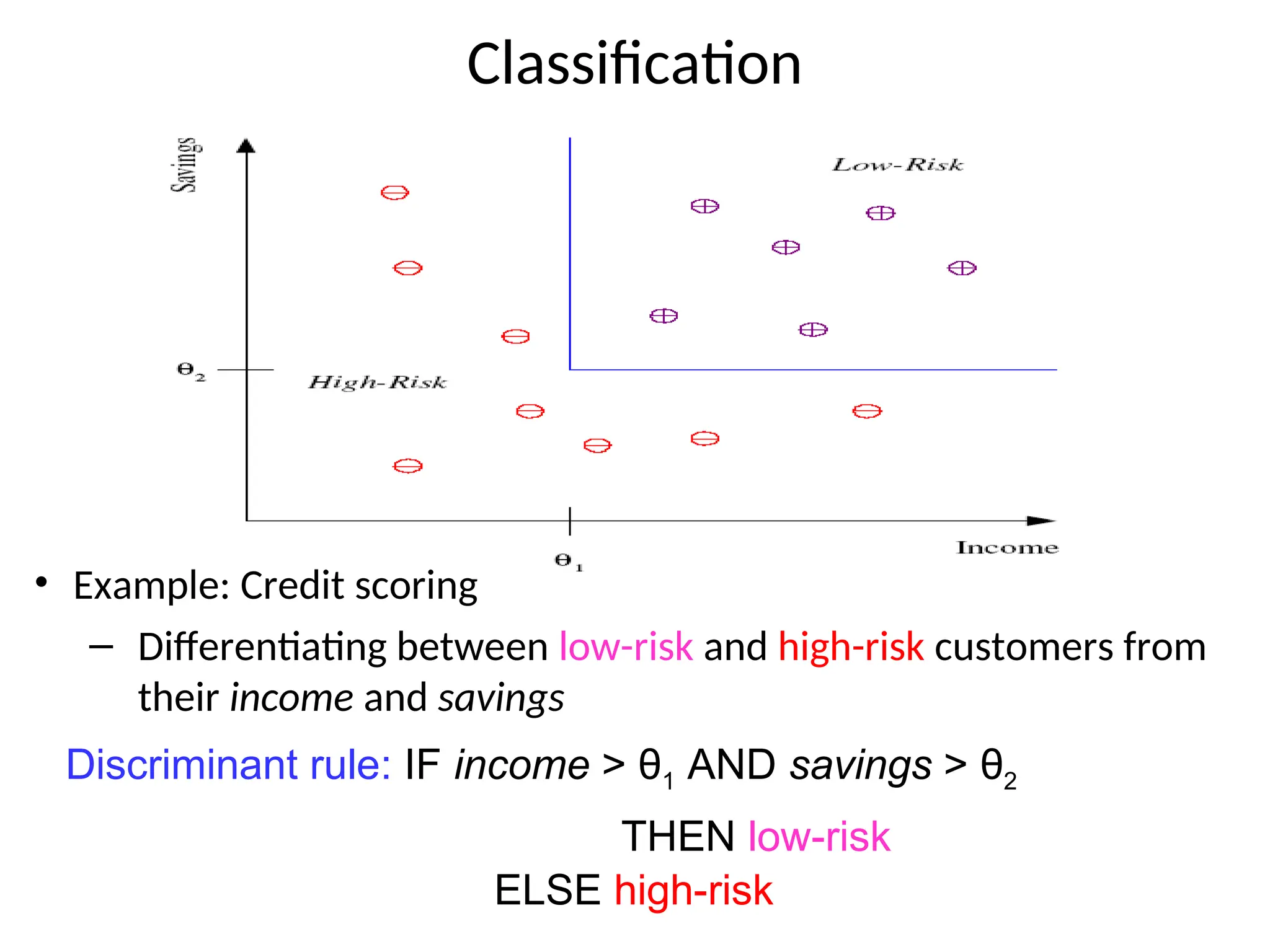
Classification
• Example: Credit scoring
– Differentiating between low-risk and high-risk customers from
their income and savings
Discriminant rule: IF income > θ1 AND savings > θ2
THEN low-risk
ELSE high-risk

Predictive Modeling: Fraud Detection
• Fraud detection or network intrusion detection
– Credit card losses in the US are over 1 billion $ per
year
– Roughly 1 in 50 transactions are fraudulent
• Approach
– Construct Model on historical data of known fraud
and non-fraud transactions
– For each new transaction estimate
p(fraudulent | transaction)
– High probability transactions investigated by fraud
police
8

DM Task: Descriptive Modeling
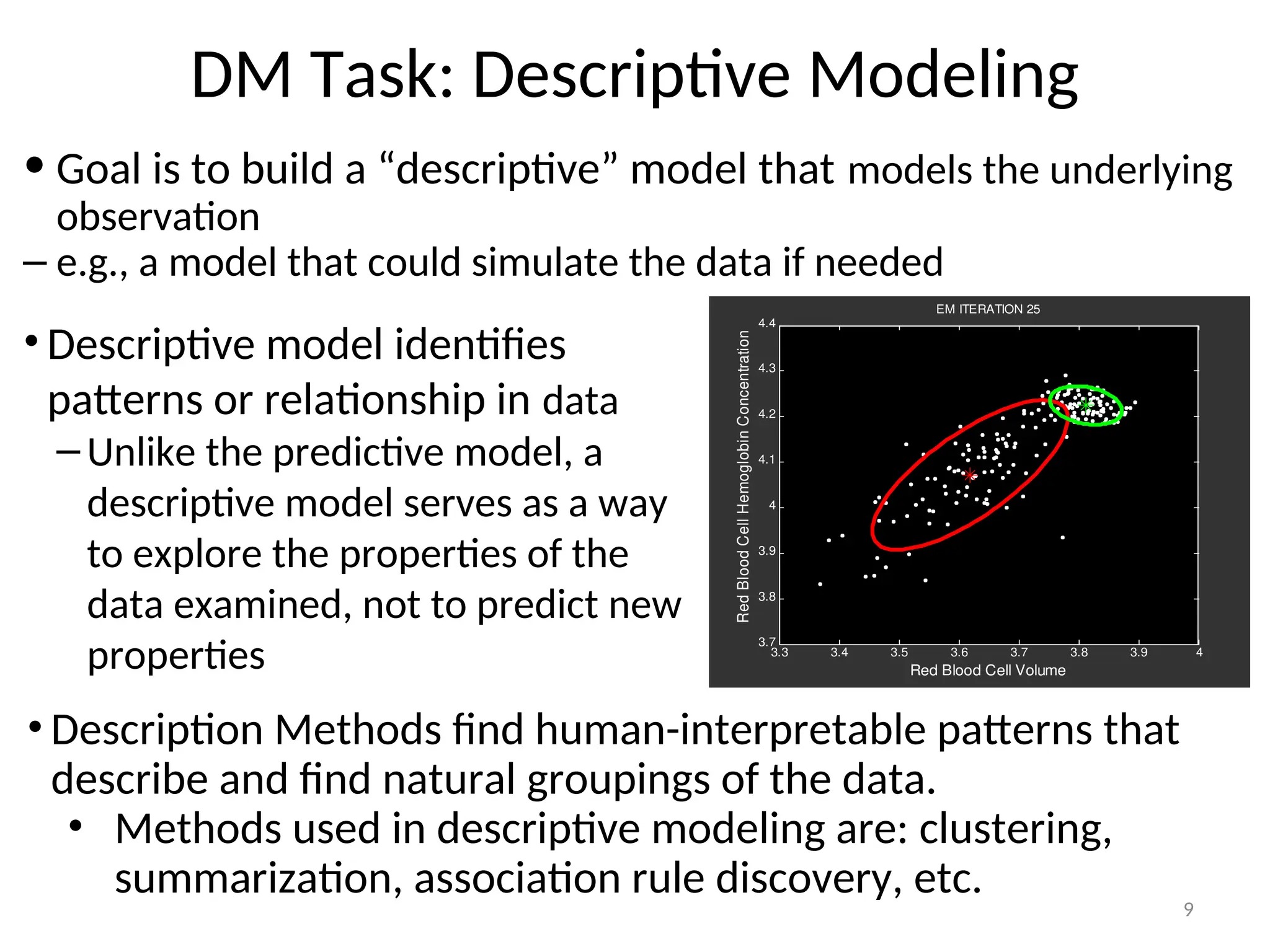
9
3.3 3.4 3.5 3.6 3.7 3.8 3.9 4
3.7
3.8
3.9
4
4.1
4.2
4.3
4.4
Red Blood Cell Volume
Red
Blood
Cell
Hemoglobin
Concentration
EM ITERATION 25
• Goal is to build a “descriptive” model that models the underlying
observation
– e.g., a model that could simulate the data if needed
• Description Methods find human-interpretable patterns that
describe and find natural groupings of the data.
• Methods used in descriptive modeling are: clustering,
summarization, association rule discovery, etc.
• Descriptive model identifies
patterns or relationship in data
– Unlike the predictive model, a
descriptive model serves as a way
to explore the properties of the
data examined, not to predict new
properties

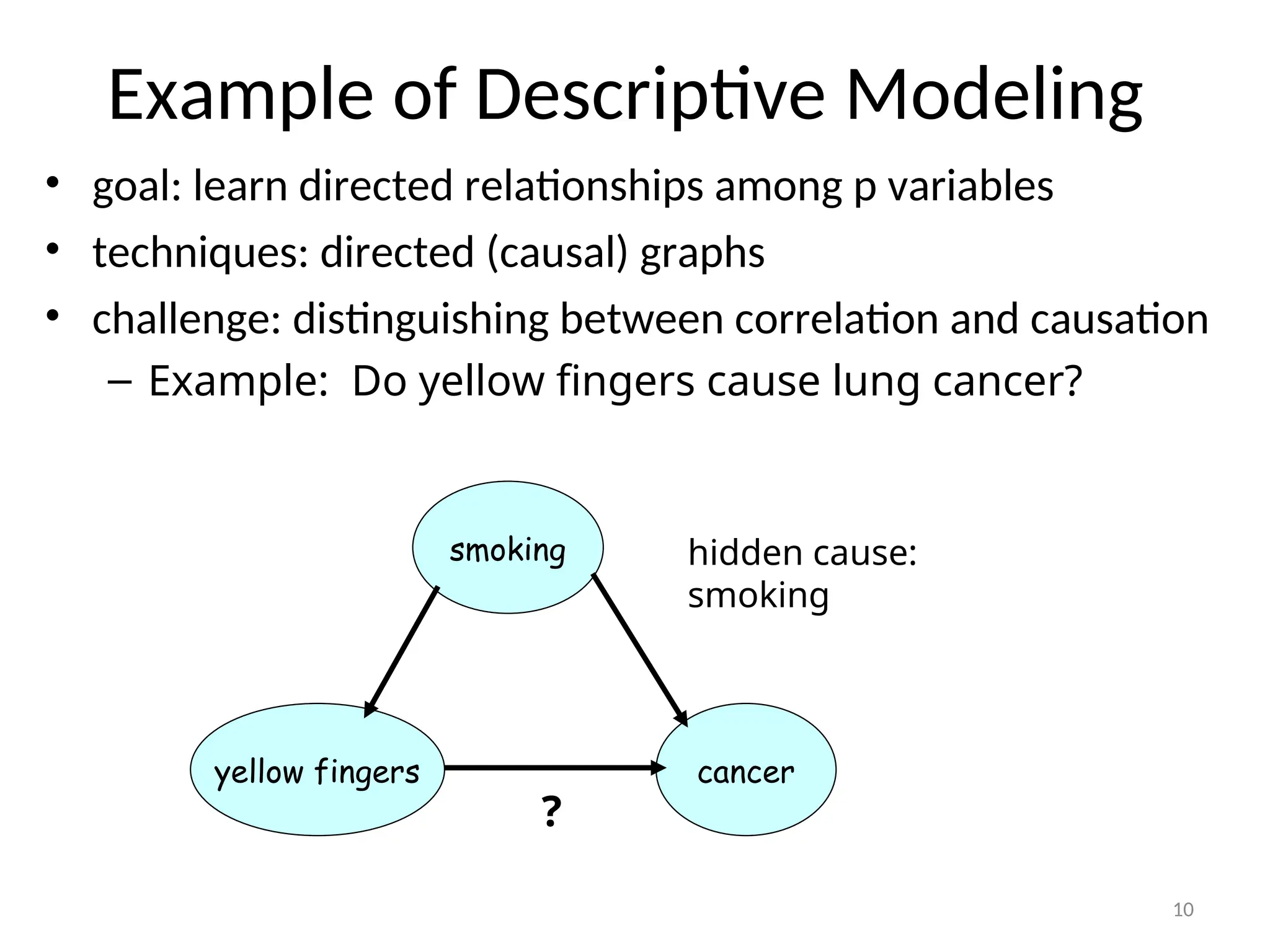
Example of Descriptive Modeling
• goal: learn directed relationships among p variables
• techniques: directed (causal) graphs
• challenge: distinguishing between correlation and causation
– Example: Do yellow fingers cause lung cancer?
cancer
yellow fingers
?
smoking hidden cause:
smoking
10

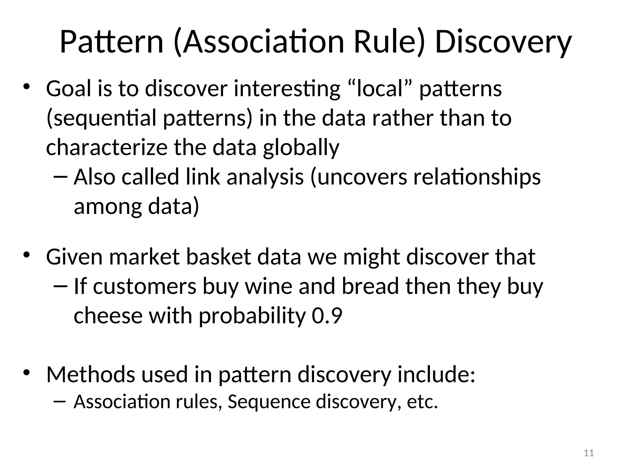
Pattern (Association Rule) Discovery
• Goal is to discover interesting “local” patterns
(sequential patterns) in the data rather than to
characterize the data globally
– Also called link analysis (uncovers relationships
among data)
• Given market basket data we might discover that
– If customers buy wine and bread then they buy
cheese with probability 0.9
• Methods used in pattern discovery include:
– Association rules, Sequence discovery, etc.
11

Basic Data Mining algorithms
• Classification (which is also called Supervised learning) maps
data into predefined groups or classes to enhance the
prediction process
• Clustering (which is also called Unsupervised learning )
groups similar data together into clusters.
– is used to find appropriate groupings of elements for a set of
data.
– Unlike classification, clustering is a kind of undirected knowledge
discovery or unsupervised learning; that is, there is no target
field, and the relationship among the data is identified by
bottom-up approach.
• Association Rule (is also known as market basket analysis)
– It discovers interesting associations between attributes
contained in a database.
– Based on frequency counts of the number of items occur in the
event, association rule tells if item X is a part of the event, then
what is the percentage of item Y is also part of the event. 14

Classification
(Supervised learning)
15
Attrib-1 Attrib-2 Attrib-3 Class
yes TRUE 2 High
No TRUE 3 High
No FALSE 5 Low
Yes FALSE 7 Low

Classification: Definition
• Classification is a data mining (machine learning) technique
used to predict group membership for data instances.
• Given a collection of records (training set), each record
contains a set of attributes, one of the attributes is the class.
– Find a model for class attribute as a function of the values of
other attributes.
• Goal: previously unseen records should be assigned a class as
accurately as possible. A test set is used to determine the
accuracy of the model.
– Usually, the given data set is divided into training and test sets,
with training set used to build the model and test set used to
validate it.
• For example, one may use classification to predict whether the
weather on a particular day will be “sunny”, “rainy” or “cloudy”.
16

17
Classification—A Two-Step Process
• Model construction: describing a set of predetermined classes
– Each tuple/sample is assumed to belong to a predefined class, as
determined by the class label attribute
– The set of tuples used for model construction is training set
– The model is represented as classification rules, decision trees,
or mathematical formulae
• Model usage: for classifying future or unknown objects
– Estimate accuracy of the model
• The known label of test sample is compared with the
classified result from the model
• Accuracy rate is the percentage of test set samples that are
correctly classified by the model
• Test set is independent of training set
– If the accuracy is acceptable, use the model to classify data
tuples whose class labels are not known

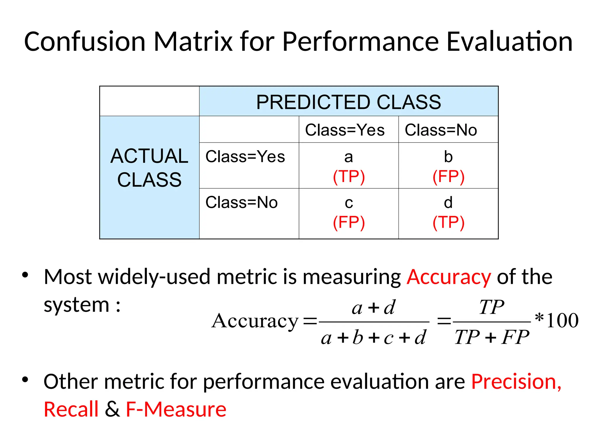
Confusion Matrix for Performance Evaluation
• Most widely-used metric is measuring Accuracy of the
system :
• Other metric for performance evaluation are Precision,
Recall & F-Measure
PREDICTED CLASS
ACTUAL
CLASS
Class=Yes Class=No
Class=Yes a
(TP)
b
(FP)
Class=No c
(FP)
d
(TP)
100
*
Accuracy
FP
TP
TP
d
c
b
a
d
a








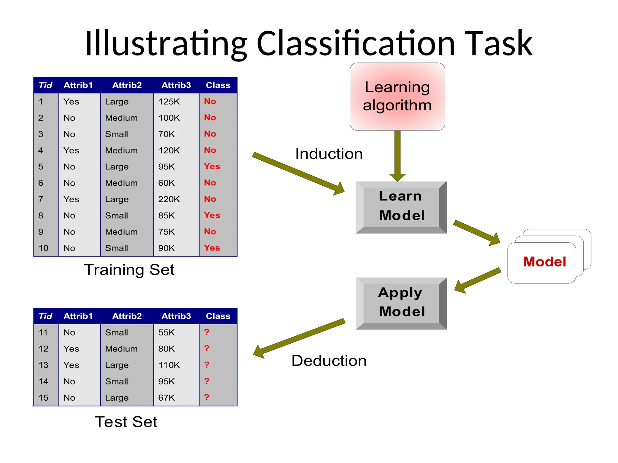
Illustrating Classification Task
Apply
Model
Induction
Deduction
Learn
Model
Model
Tid Attrib1 Attrib2 Attrib3 Class
1 Yes Large 125K No
2 No Medium 100K No
3 No Small 70K No
4 Yes Medium 120K No
5 No Large 95K Yes
6 No Medium 60K No
7 Yes Large 220K No
8 No Small 85K Yes
9 No Medium 75K No
10 No Small 90K Yes
10
Tid Attrib1 Attrib2 Attrib3 Class
11 No Small 55K ?
12 Yes Medium 80K ?
13 Yes Large 110K ?
14 No Small 95K ?
15 No Large 67K ?
10
Test Set
Learning
algorithm
Training Set

Classification methods
• Goal: Predict class Ci = f(x1, x2, .. xn)
• There are various classification methods.
Popular classification techniques include the
following.
– K-nearest neighbor
– Decision tree classifier: divide decision space into
piecewise constant regions.
– Neural networks: partition by non-linear boundaries
– Bayesian network: a probabilistic model
– Support vector machine
20

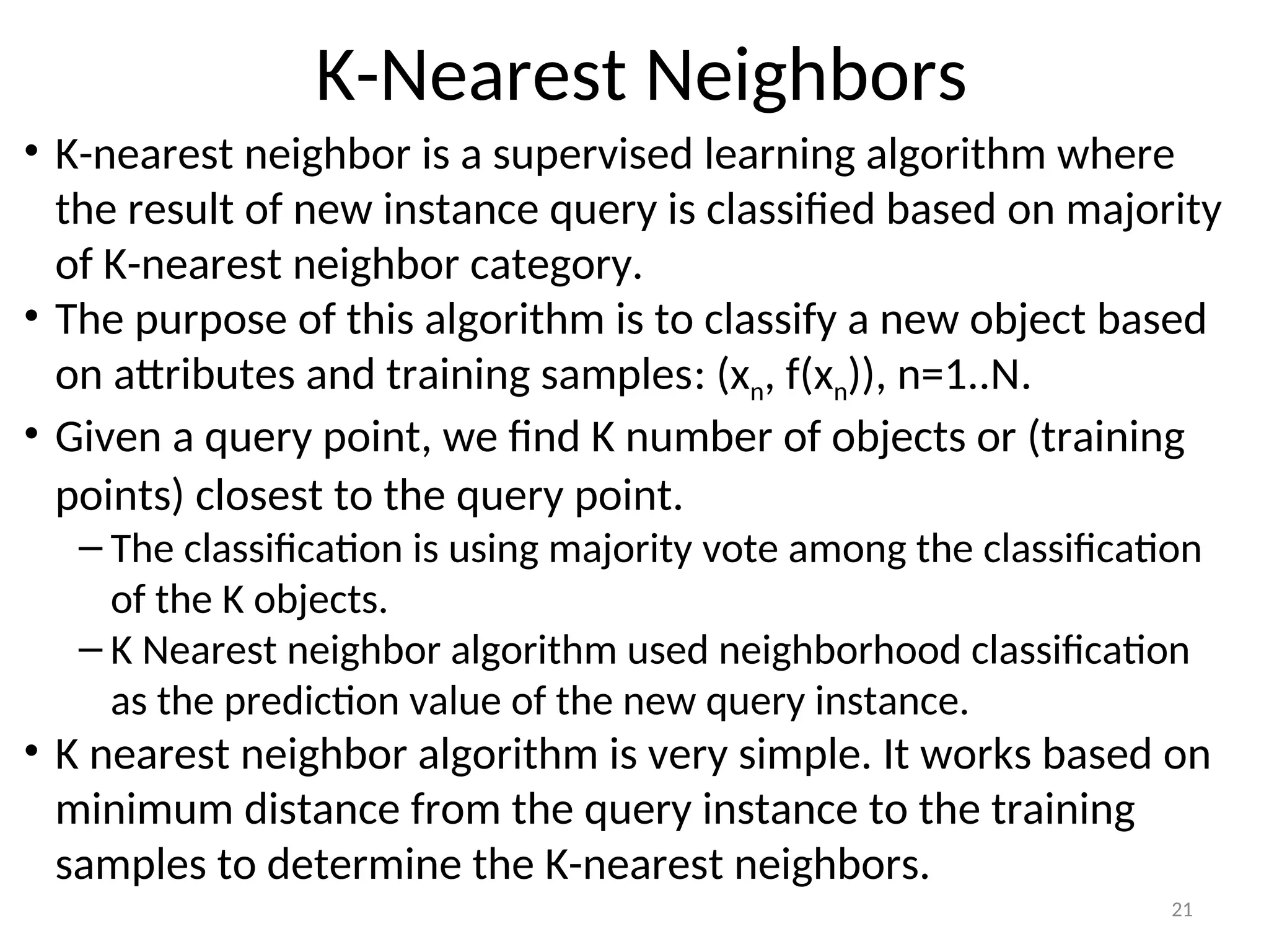
K-Nearest Neighbors
• K-nearest neighbor is a supervised learning algorithm where
the result of new instance query is classified based on majority
of K-nearest neighbor category.
• The purpose of this algorithm is to classify a new object based
on attributes and training samples: (xn, f(xn)), n=1..N.
• Given a query point, we find K number of objects or (training
points) closest to the query point.
– The classification is using majority vote among the classification
of the K objects.
– K Nearest neighbor algorithm used neighborhood classification
as the prediction value of the new query instance.
• K nearest neighbor algorithm is very simple. It works based on
minimum distance from the query instance to the training
samples to determine the K-nearest neighbors.
21

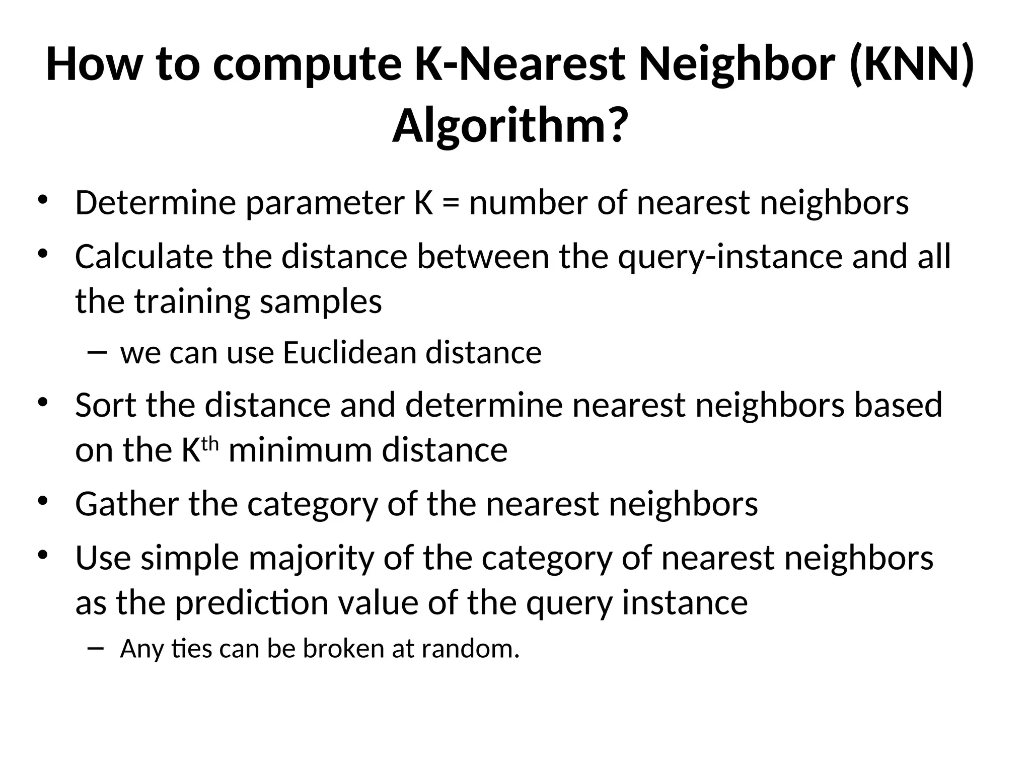
How to compute K-Nearest Neighbor (KNN)
Algorithm?
• Determine parameter K = number of nearest neighbors
• Calculate the distance between the query-instance and all
the training samples
– we can use Euclidean distance
• Sort the distance and determine nearest neighbors based
on the Kth
minimum distance
• Gather the category of the nearest neighbors
• Use simple majority of the category of nearest neighbors
as the prediction value of the query instance
– Any ties can be broken at random.

23
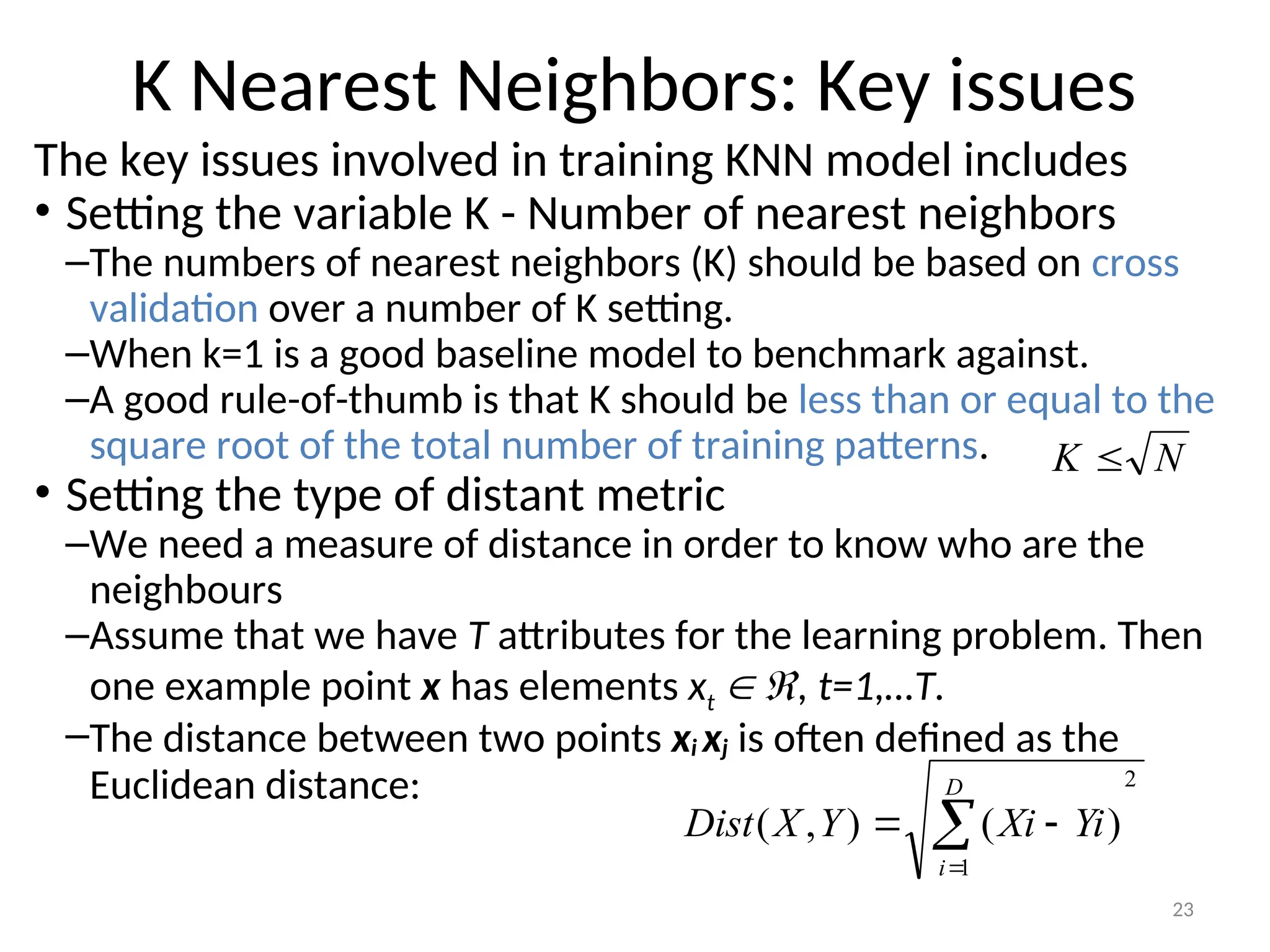
K Nearest Neighbors: Key issues
The key issues involved in training KNN model includes
• Setting the variable K - Number of nearest neighbors
–The numbers of nearest neighbors (K) should be based on cross
validation over a number of K setting.
–When k=1 is a good baseline model to benchmark against.
–A good rule-of-thumb is that K should be less than or equal to the
square root of the total number of training patterns.
• Setting the type of distant metric
–We need a measure of distance in order to know who are the
neighbours
–Assume that we have T attributes for the learning problem. Then
one example point x has elements xt  , t=1,…T.
–The distance between two points xi xj is often defined as the
Euclidean distance: 2
1
)
(
)
,
( 



D
i
Yi
Xi
Y
X
Dist
N
K 

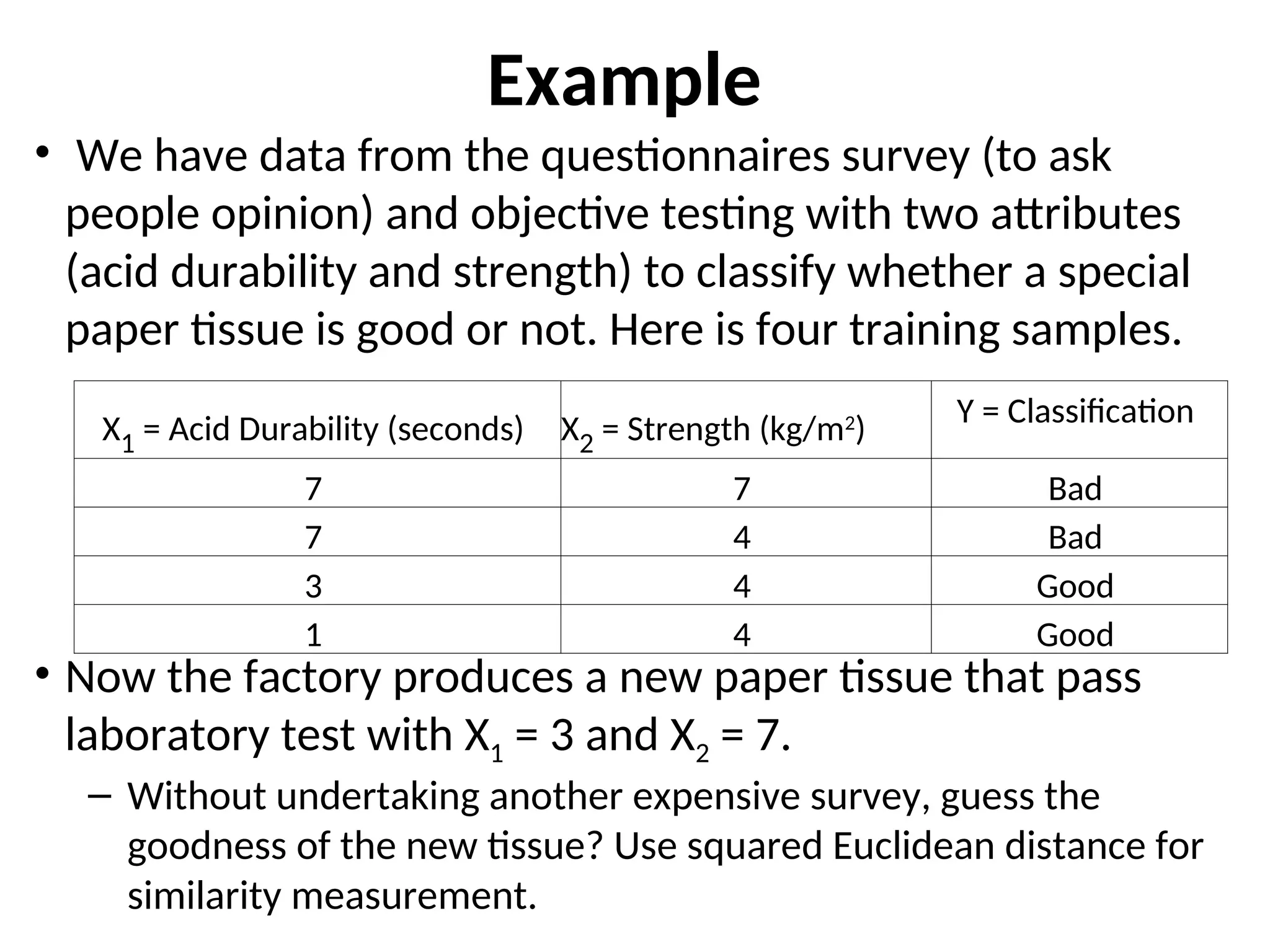
Example
• We have data from the questionnaires survey (to ask
people opinion) and objective testing with two attributes
(acid durability and strength) to classify whether a special
paper tissue is good or not. Here is four training samples.
• Now the factory produces a new paper tissue that pass
laboratory test with X1 = 3 and X2 = 7.
– Without undertaking another expensive survey, guess the
goodness of the new tissue? Use squared Euclidean distance for
similarity measurement.
X1 = Acid Durability (seconds) X2 = Strength (kg/m2
)
Y = Classification
7 7 Bad
7 4 Bad
3 4 Good
1 4 Good

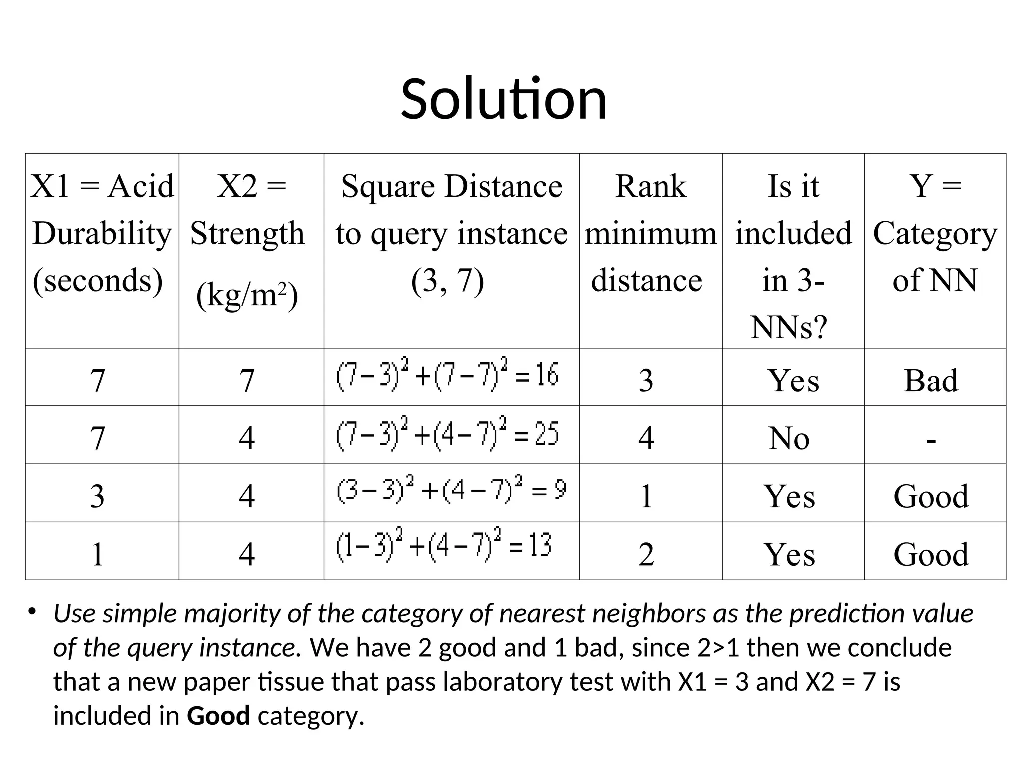
Solution
X1 = Acid
Durability
(seconds)
X2 =
Strength
(kg/m2
)
Square Distance
to query instance
(3, 7)
Rank
minimum
distance
Is it
included
in 3-
NNs?
Y =
Category
of NN
7 7 3 Yes Bad
7 4 4 No -
3 4 1 Yes Good
1 4 2 Yes Good
• Use simple majority of the category of nearest neighbors as the prediction value
of the query instance. We have 2 good and 1 bad, since 2>1 then we conclude
that a new paper tissue that pass laboratory test with X1 = 3 and X2 = 7 is
included in Good category.

27
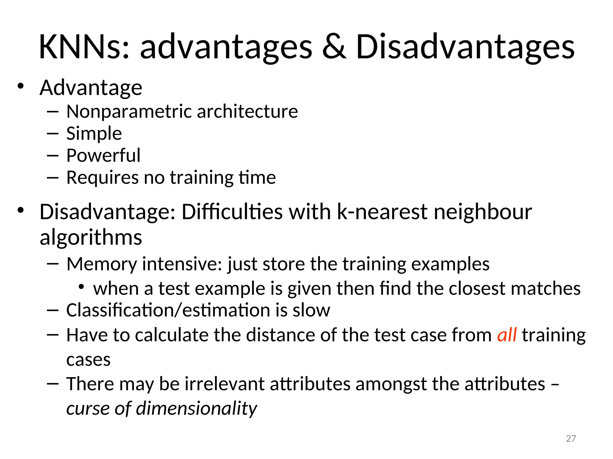
KNNs: advantages & Disadvantages
• Advantage
– Nonparametric architecture
– Simple
– Powerful
– Requires no training time
• Disadvantage: Difficulties with k-nearest neighbour
algorithms
– Memory intensive: just store the training examples
• when a test example is given then find the closest matches
– Classification/estimation is slow
– Have to calculate the distance of the test case from all training
cases
– There may be irrelevant attributes amongst the attributes –
curse of dimensionality

Decision Trees
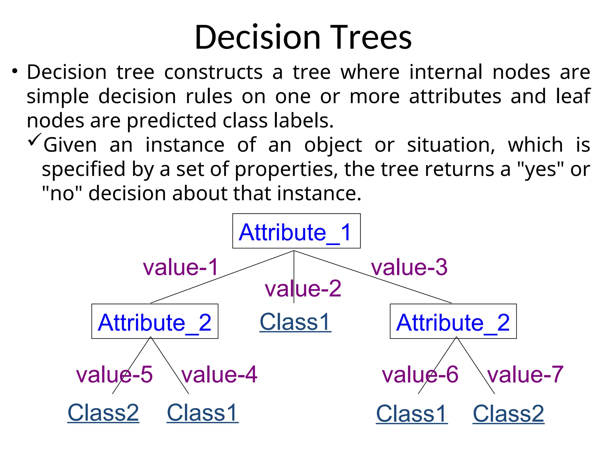
• Decision tree constructs a tree where internal nodes are
simple decision rules on one or more attributes and leaf
nodes are predicted class labels.
Given an instance of an object or situation, which is
specified by a set of properties, the tree returns a "yes" or
"no" decision about that instance.
Attribute_1
Attribute_2 Attribute_2
value-1
value-2
value-3
Class1
Class1
Class2 Class2
Class1
value-5 value-4 value-6 value-7

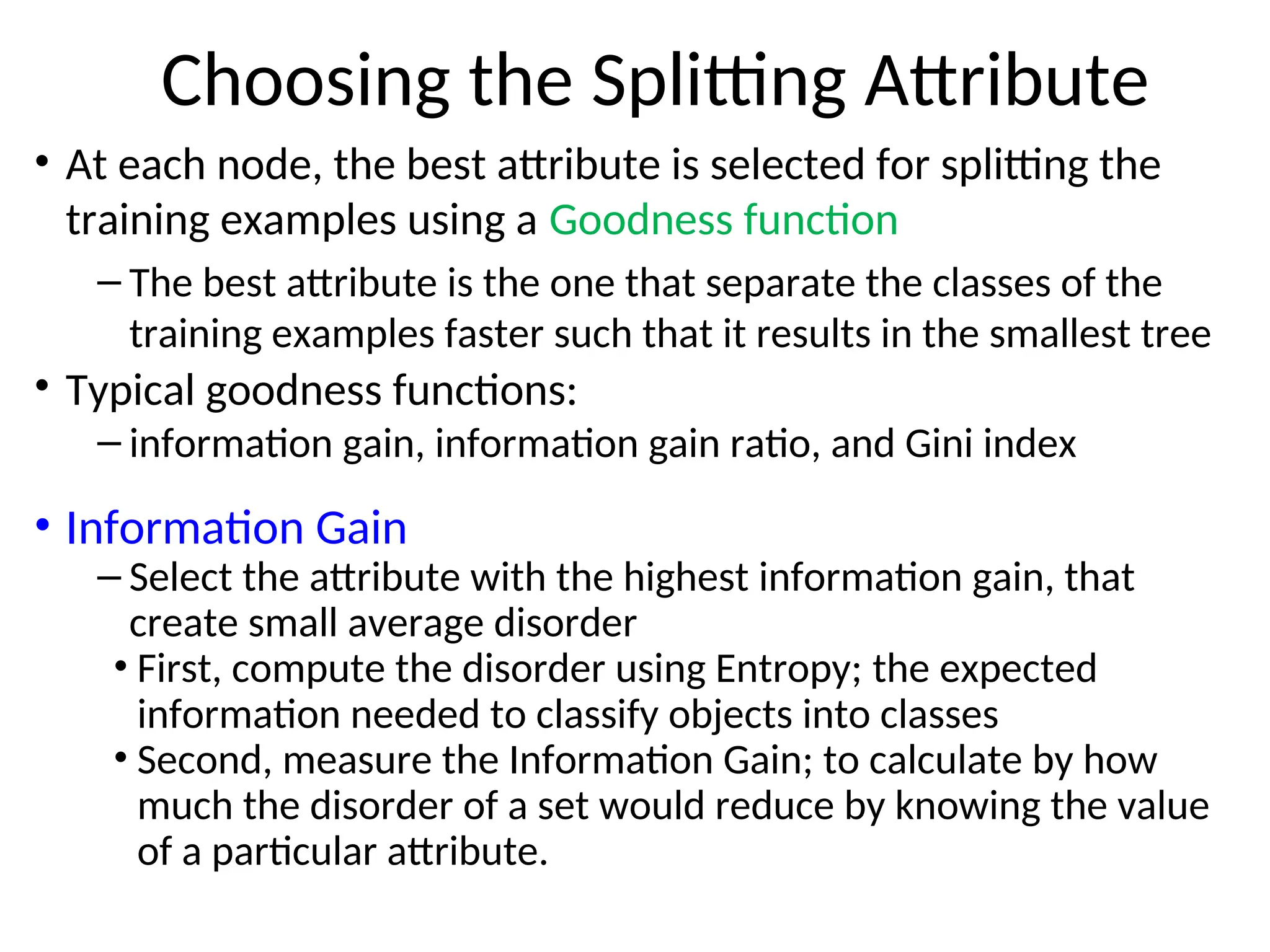
Choosing the Splitting Attribute
• At each node, the best attribute is selected for splitting the
training examples using a Goodness function
– The best attribute is the one that separate the classes of the
training examples faster such that it results in the smallest tree
• Typical goodness functions:
– information gain, information gain ratio, and Gini index
• Information Gain
– Select the attribute with the highest information gain, that
create small average disorder
• First, compute the disorder using Entropy; the expected
information needed to classify objects into classes
• Second, measure the Information Gain; to calculate by how
much the disorder of a set would reduce by knowing the value
of a particular attribute.

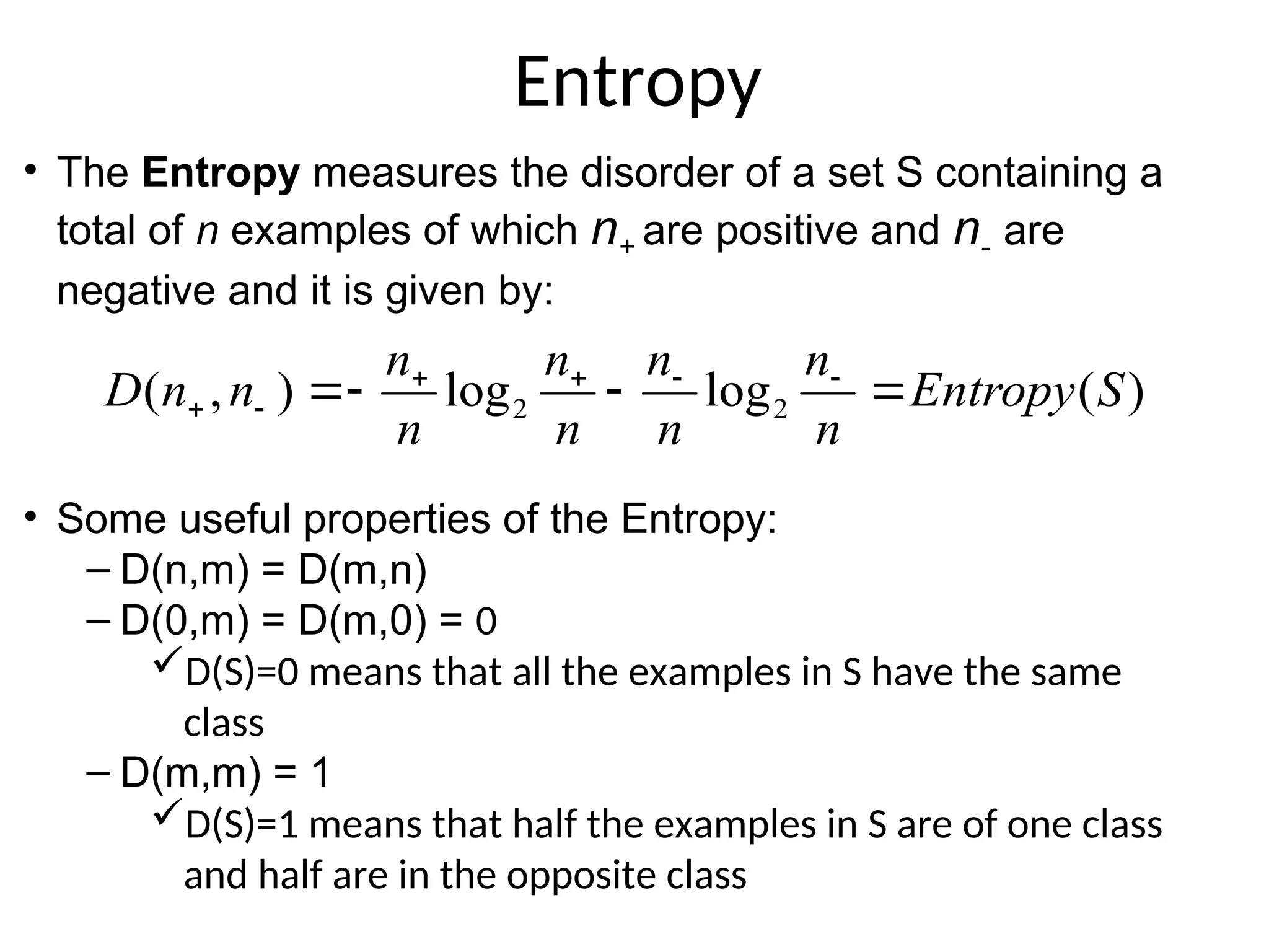
Entropy
)
(
log
log
)
,
( 2
2 S
Entropy
n
n
n
n
n
n
n
n
n
n
D 


 





• The Entropy measures the disorder of a set S containing a
total of n examples of which n+ are positive and n- are
negative and it is given by:
• Some useful properties of the Entropy:
– D(n,m) = D(m,n)
– D(0,m) = D(m,0) = 0
D(S)=0 means that all the examples in S have the same
class
– D(m,m) = 1
D(S)=1 means that half the examples in S are of one class
and half are in the opposite class

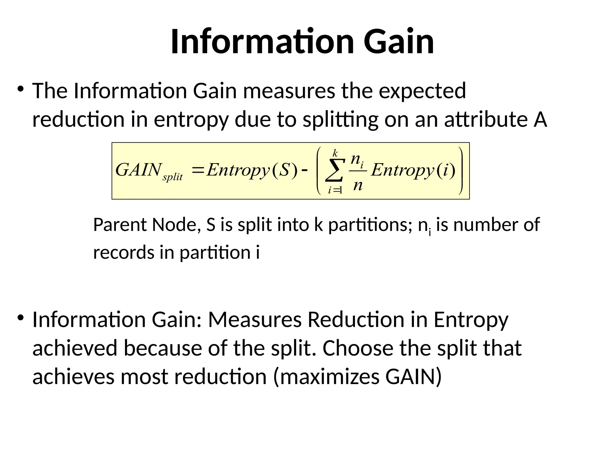
Information Gain
• The Information Gain measures the expected
reduction in entropy due to splitting on an attribute A
Parent Node, S is split into k partitions; ni is number of
records in partition i
• Information Gain: Measures Reduction in Entropy
achieved because of the split. Choose the split that
achieves most reduction (maximizes GAIN)







 

k
i
i
split i
Entropy
n
n
S
Entropy
GAIN
1
)
(
)
(

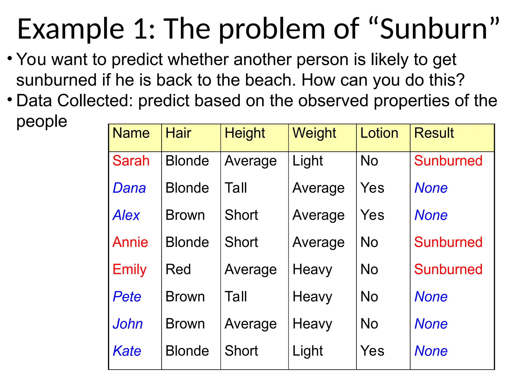
Example 1: The problem of “Sunburn”
• You want to predict whether another person is likely to get
sunburned if he is back to the beach. How can you do this?
• Data Collected: predict based on the observed properties of the
people
Name Hair Height Weight Lotion Result
Sarah Blonde Average Light No Sunburned
Dana Blonde Tall Average Yes None
Alex Brown Short Average Yes None
Annie Blonde Short Average No Sunburned
Emily Red Average Heavy No Sunburned
Pete Brown Tall Heavy No None
John Brown Average Heavy No None
Kate Blonde Short Light Yes None

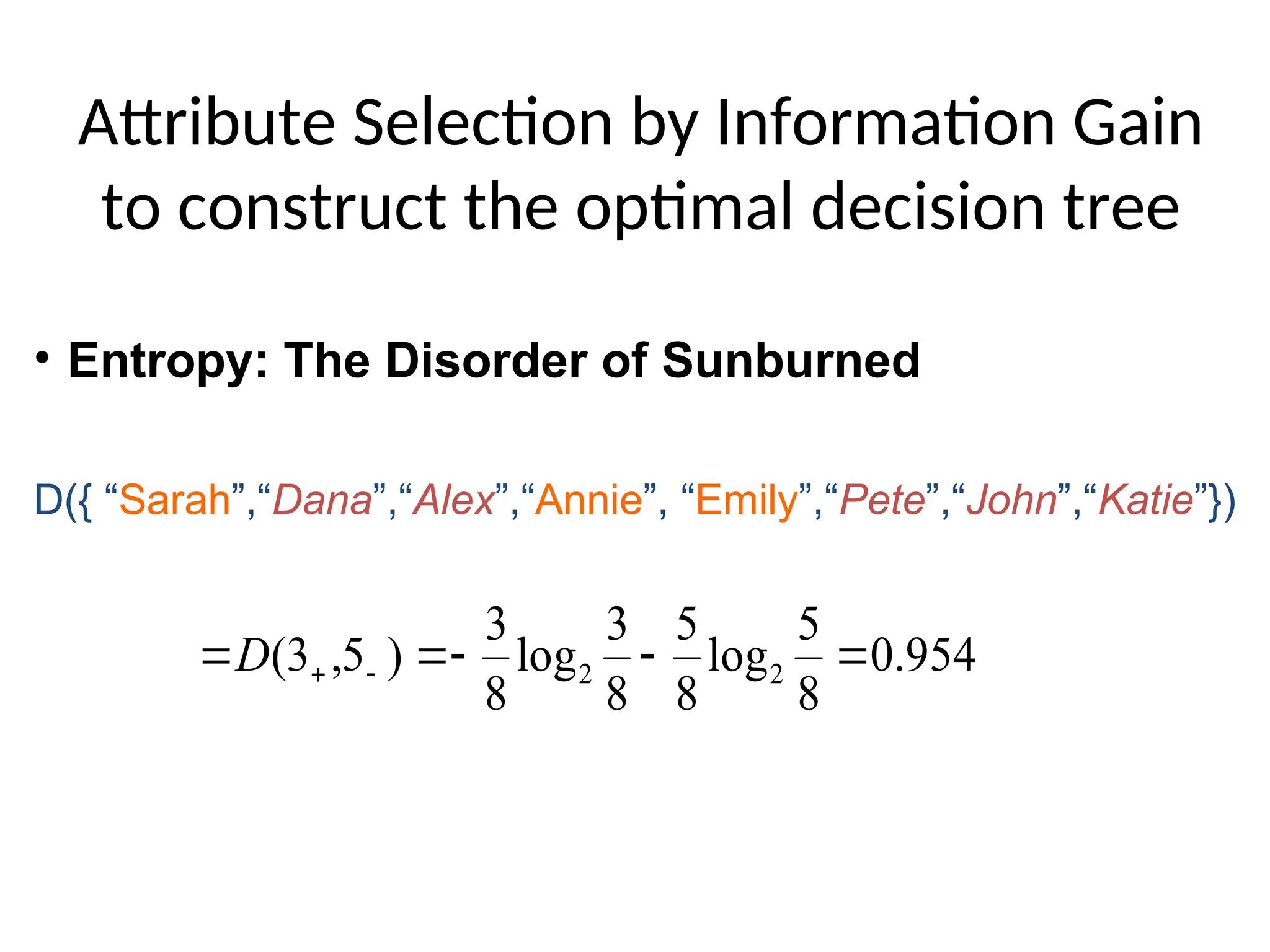
Attribute Selection by Information Gain
to construct the optimal decision tree
954
.
0
8
5
log
8
5
8
3
log
8
3
)
5
,
3
( 2
2 



 

D
D({ “Sarah”,“Dana”,“Alex”,“Annie”, “Emily”,“Pete”,“John”,“Katie”})
• Entropy: The Disorder of Sunburned

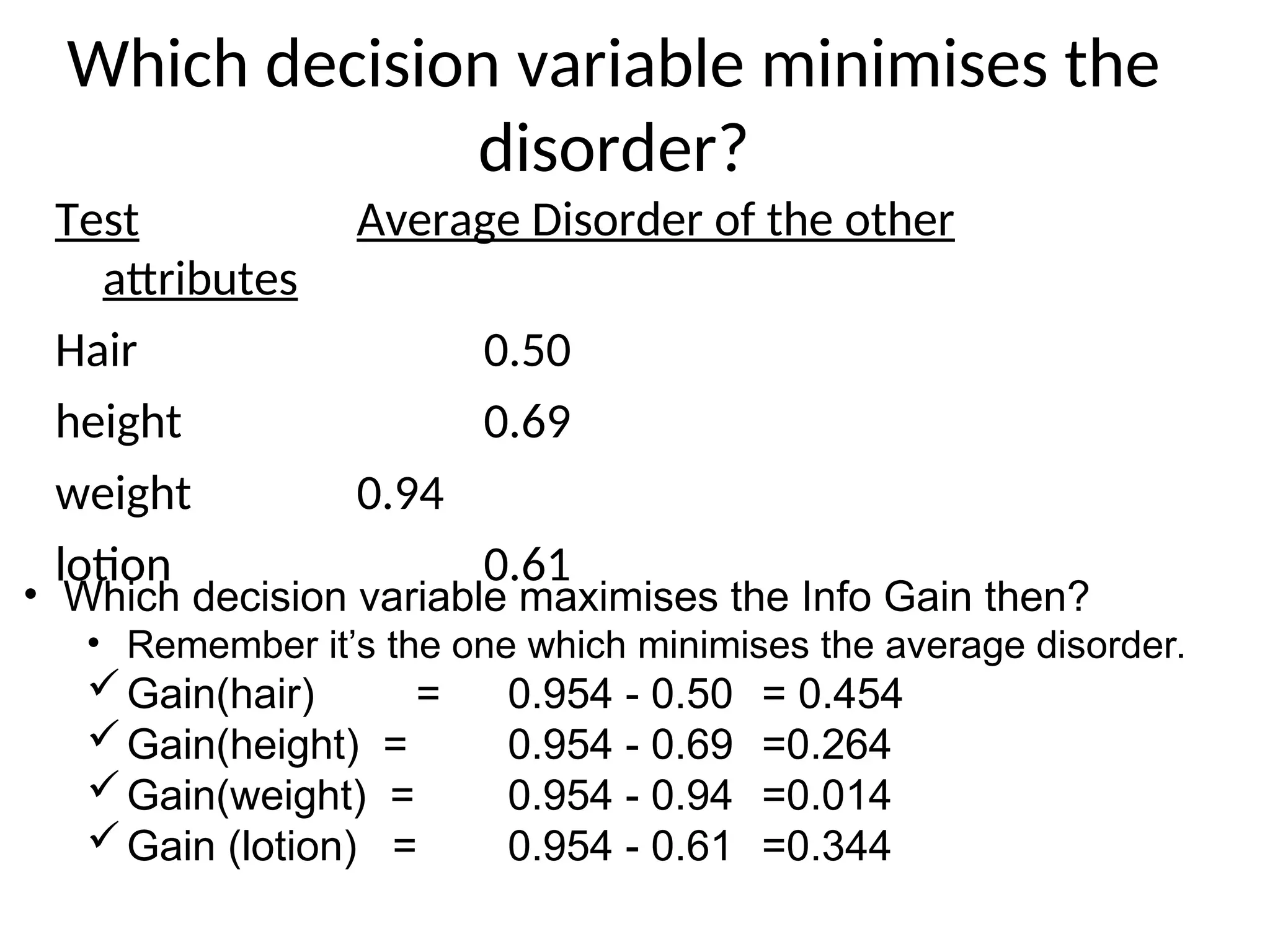
Which decision variable minimises the
disorder?
Test Average Disorder of the other
attributes
Hair 0.50
height 0.69
weight 0.94
lotion 0.61
• Which decision variable maximises the Info Gain then?
• Remember it’s the one which minimises the average disorder.
Gain(hair) = 0.954 - 0.50 = 0.454
Gain(height) = 0.954 - 0.69 =0.264
Gain(weight) = 0.954 - 0.94 =0.014
Gain (lotion) = 0.954 - 0.61 =0.344

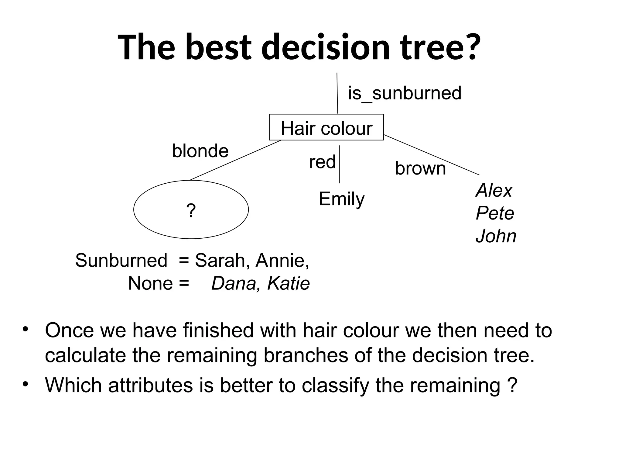
The best decision tree?
?
is_sunburned
Alex
Pete
John
Emily
Sunburned = Sarah, Annie,
None = Dana, Katie
Hair colour
brown
blonde
red
• Once we have finished with hair colour we then need to
calculate the remaining branches of the decision tree.
• Which attributes is better to classify the remaining ?

The best Decision Tree
Sarah,
Annie
is_sunburned
Alex,
Pete,
John
Emily
Dana,
Katie
Hair colour
Lotion used
blonde
red
brown
no yes
• This is the simplest and optimal one possible and it makes a
lot of sense.
• It classifies 4 of the people on just the hair colour alone.

Sunburn sufferers are ...
• You can view Decision Tree as an IF-THEN_ELSE
statement which tells us whether someone will suffer
from sunburn.
If (Hair-Colour=“red”) then
return (sunburned = yes)
else if (hair-colour=“blonde” and lotion-
used=“No”) then
return (sunburned = yes)
else
return (false)

Why decision tree induction in DM?
Cons
Cannot handle complicated
relationship between
features
Simple decision boundaries
Problems with lots of missing
data
Pros
+ Reasonable training time
+ Fast application
+ Easy to interpret
+ Easy to implement
+Can handle large number
of features
46
• Relatively faster learning speed (than other classification
methods)
• Convertible to simple and easy to understand classification if-
then-else rules
• Comparable classification accuracy with other methods
• Does not require any prior knowledge of data distribution,
works well on noisy data.

48
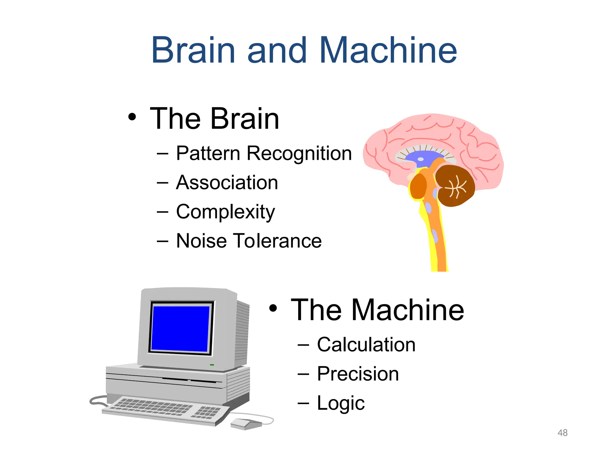
Brain and Machine
• The Brain
– Pattern Recognition
– Association
– Complexity
– Noise Tolerance
• The Machine
– Calculation
– Precision
– Logic

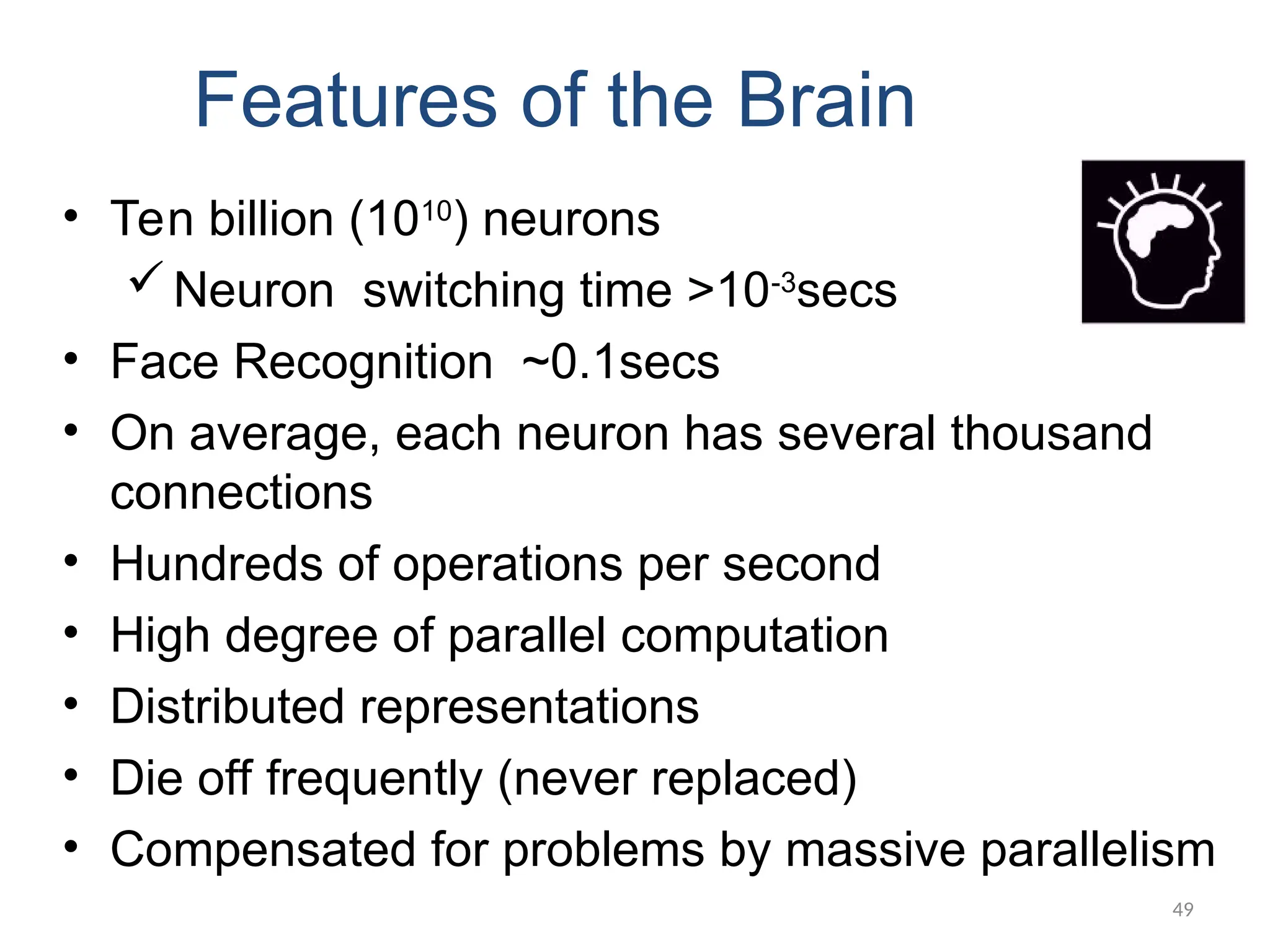
49
Features of the Brain
• Ten billion (1010
) neurons
Neuron switching time >10-3
secs
• Face Recognition ~0.1secs
• On average, each neuron has several thousand
connections
• Hundreds of operations per second
• High degree of parallel computation
• Distributed representations
• Die off frequently (never replaced)
• Compensated for problems by massive parallelism

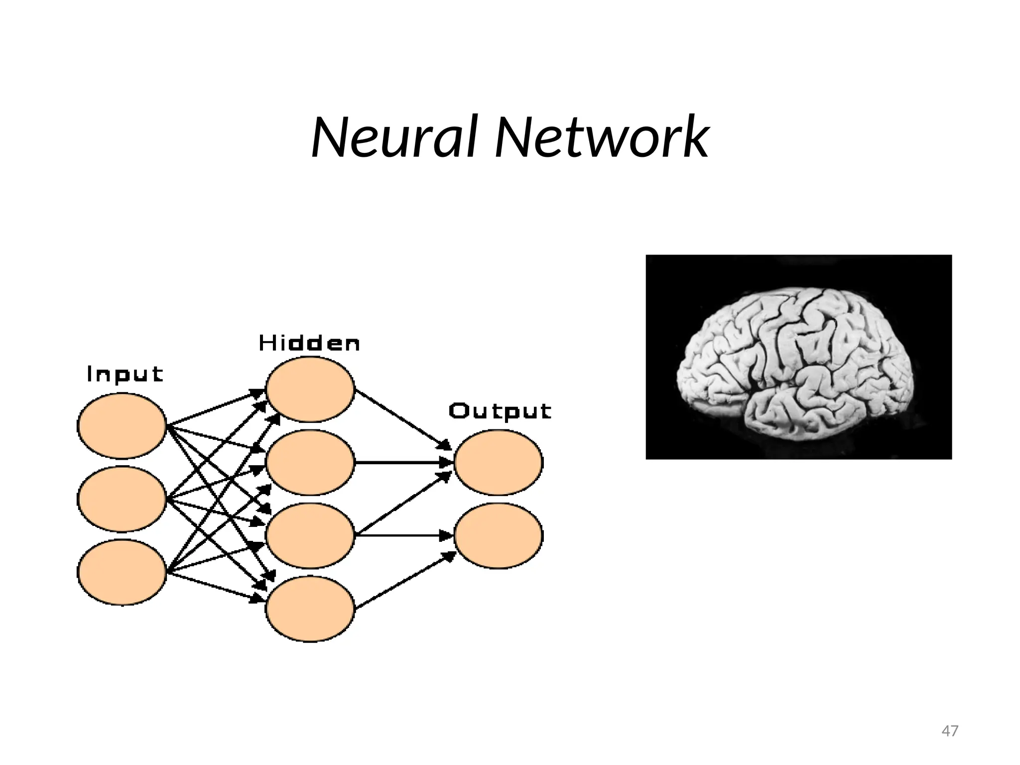
Neural Network classifier
• It is represented as a layered set of interconnected
processors. These processor nodes has a relationship
with the neurons of the brain. Each node has a weighted
connection to several other nodes in adjacent layers.
Individual nodes take the input received from
connected nodes and use the weights together to
compute output values.
• The inputs are fed simultaneously into the input layer.
• The weighted outputs of these units are fed into hidden
layer.
• The weighted outputs of the last hidden layer are inputs
to units making up the output layer.
50

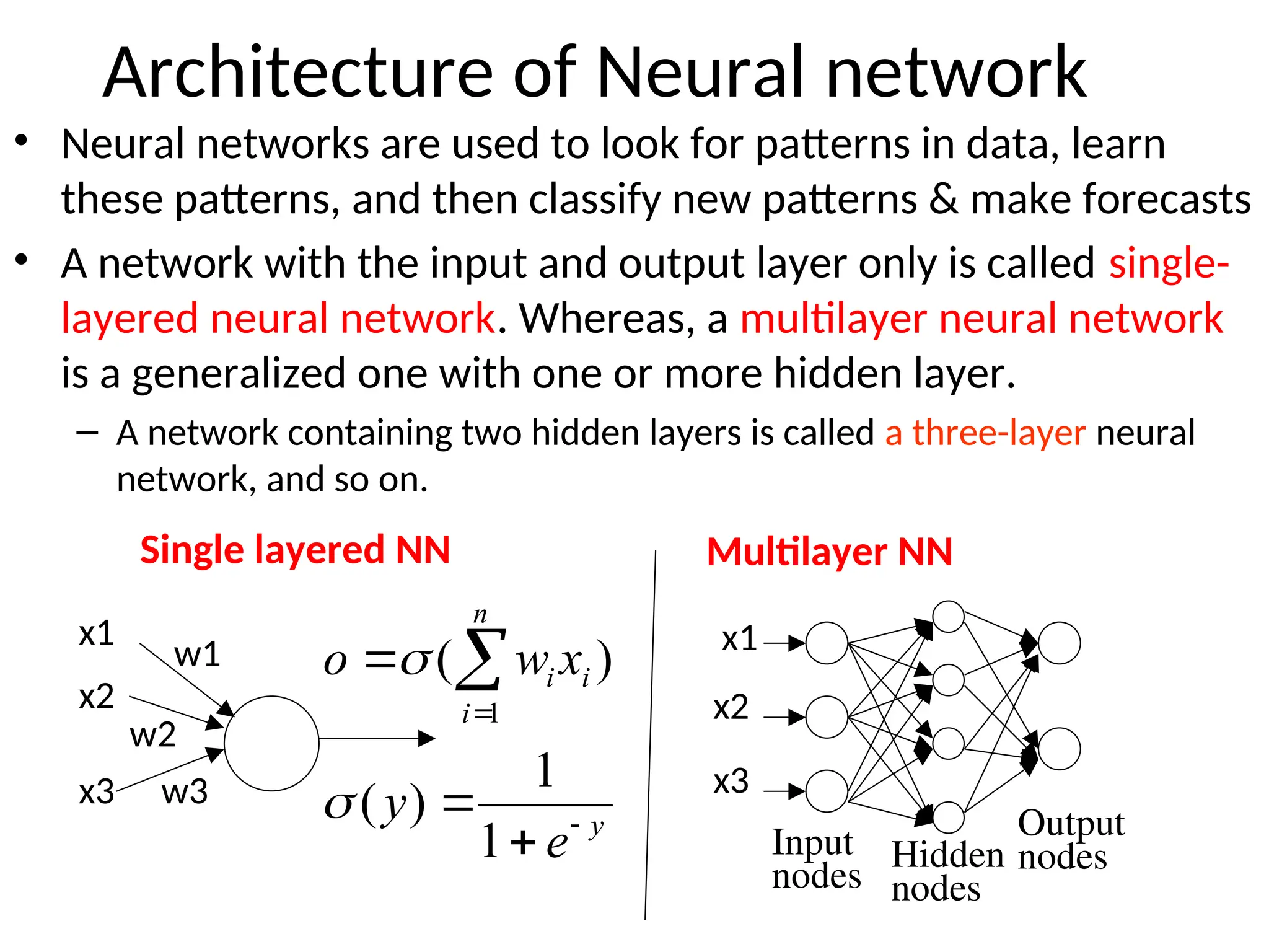
Architecture of Neural network
• Neural networks are used to look for patterns in data, learn
these patterns, and then classify new patterns & make forecasts
• A network with the input and output layer only is called single-
layered neural network. Whereas, a multilayer neural network
is a generalized one with one or more hidden layer.
– A network containing two hidden layers is called a three-layer neural
network, and so on.
Hidden
nodes
Output
nodes
x1
x2
x3
x1
x2
x3
w1
w2
w3
y
n
i
i
i
e
y
x
w
o




 
1
1
)
(
)
(
1


Single layered NN Multilayer NN
Input
nodes

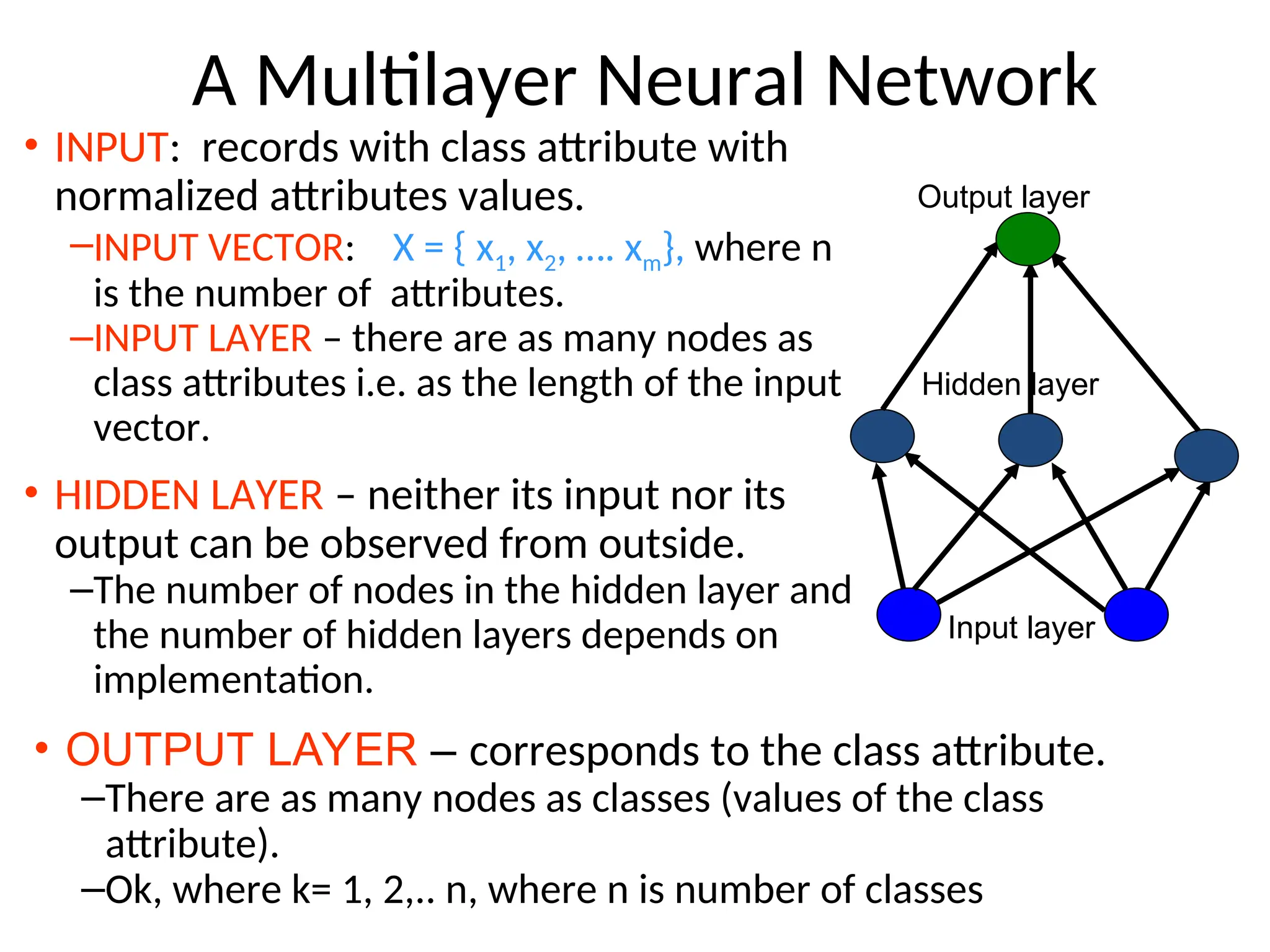
A Multilayer Neural Network
• INPUT: records with class attribute with
normalized attributes values.
–INPUT VECTOR: X = { x1, x2, …. xm}, where n
is the number of attributes.
–INPUT LAYER – there are as many nodes as
class attributes i.e. as the length of the input
vector.
• HIDDEN LAYER – neither its input nor its
output can be observed from outside.
–The number of nodes in the hidden layer and
the number of hidden layers depends on
implementation.
Input layer
Hidden layer
Output layer
• OUTPUT LAYER – corresponds to the class attribute.
–There are as many nodes as classes (values of the class
attribute).
–Ok, where k= 1, 2,.. n, where n is number of classes

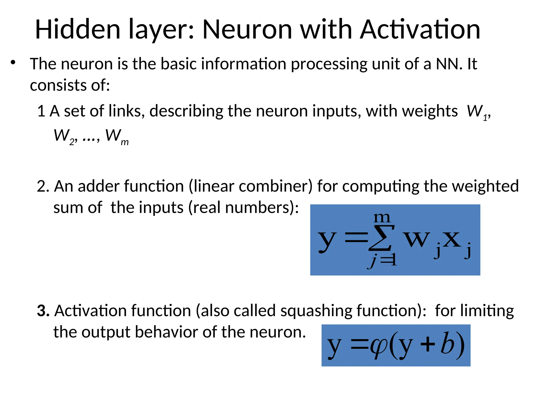
Hidden layer: Neuron with Activation
• The neuron is the basic information processing unit of a NN. It
consists of:
1 A set of links, describing the neuron inputs, with weights W1,
W2, …, Wm
2. An adder function (linear combiner) for computing the weighted
sum of the inputs (real numbers):
3. Activation function (also called squashing function): for limiting
the output behavior of the neuron.



m
1
j
jx
w
y
j
)
(y
y b



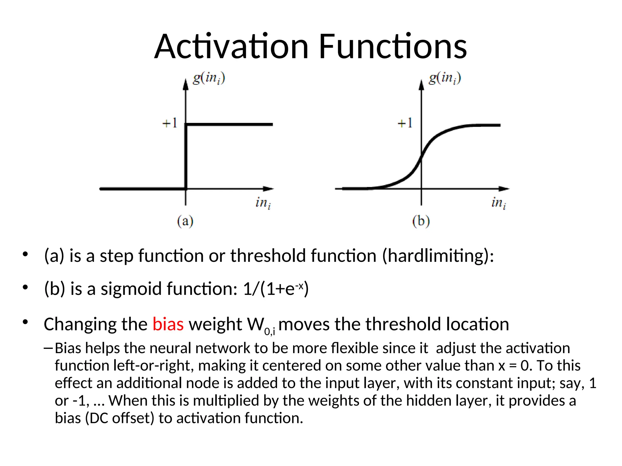
Activation Functions
• (a) is a step function or threshold function (hardlimiting):
• (b) is a sigmoid function: 1/(1+e-x
)
• Changing the bias weight W0,i moves the threshold location
–Bias helps the neural network to be more flexible since it adjust the activation
function left-or-right, making it centered on some other value than x = 0. To this
effect an additional node is added to the input layer, with its constant input; say, 1
or -1, … When this is multiplied by the weights of the hidden layer, it provides a
bias (DC offset) to activation function.

Two Topologies of neural network
• NN can be designed in a feed forward or recurrent
manner
• In a feed forward neural network connections
between the units do not form a directed cycle.
– In this network, the information moves in only one
direction, forward, from the input nodes, through the
hidden nodes (if any) & to the output nodes. There are
no cycles or loops or no feedback connections are
present in the network, that is, connections extending
from outputs of units to inputs of units in the same
layer or previous layers.
• In recurrent networks data circulates back &
forth until the activation of the units is stabilized
– Recurrent networks have a feedback loop where data
can be fed back into the input at some point before it is
fed forward again for further processing and final
output.
56

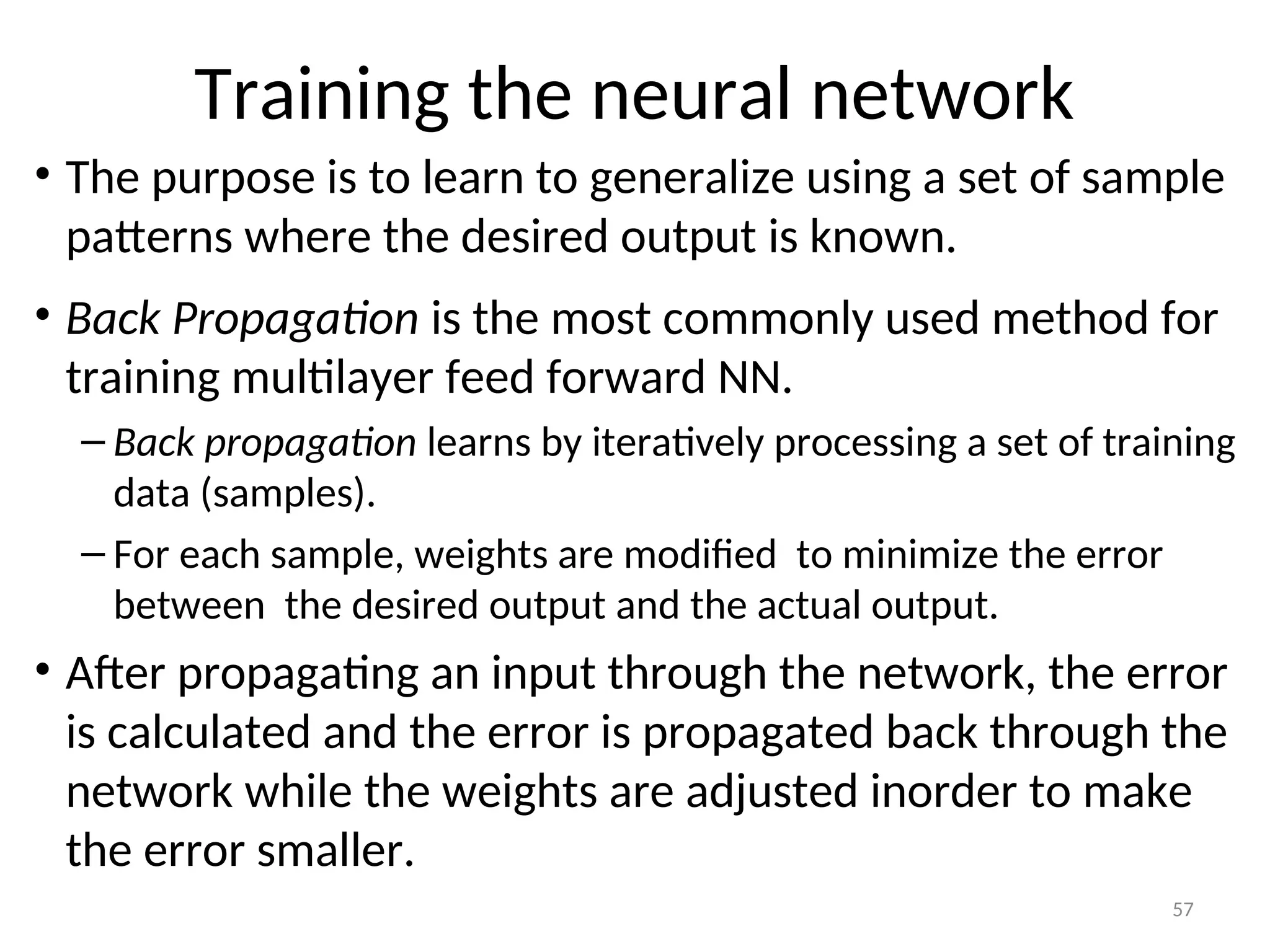
Training the neural network
• The purpose is to learn to generalize using a set of sample
patterns where the desired output is known.
• Back Propagation is the most commonly used method for
training multilayer feed forward NN.
– Back propagation learns by iteratively processing a set of training
data (samples).
– For each sample, weights are modified to minimize the error
between the desired output and the actual output.
• After propagating an input through the network, the error
is calculated and the error is propagated back through the
network while the weights are adjusted inorder to make
the error smaller.
57

Training Algorithm
•The applied learning algorithm is as follows
–Initialize the weights and threshold to small random
numbers.
–Present a vector x to the neuron inputs and calculate the
output using the adder function.
–Apply the activation function such that
–Update the weights according to the error.
j
T
j
j x
y
y
W
W *
)
(
* 

 



m
1
j
jx
w
y
j







 0
y
if
1
0
y
if
0
y

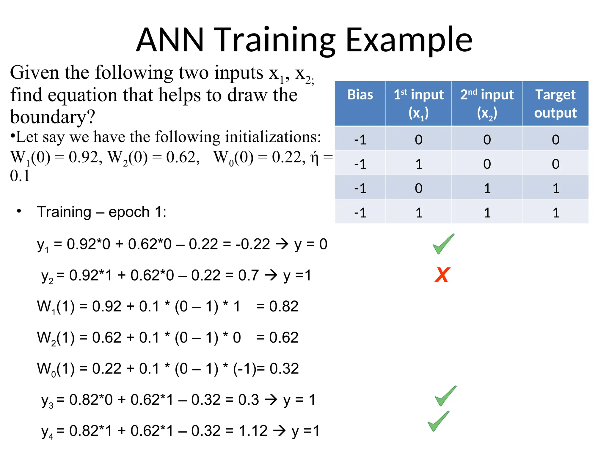
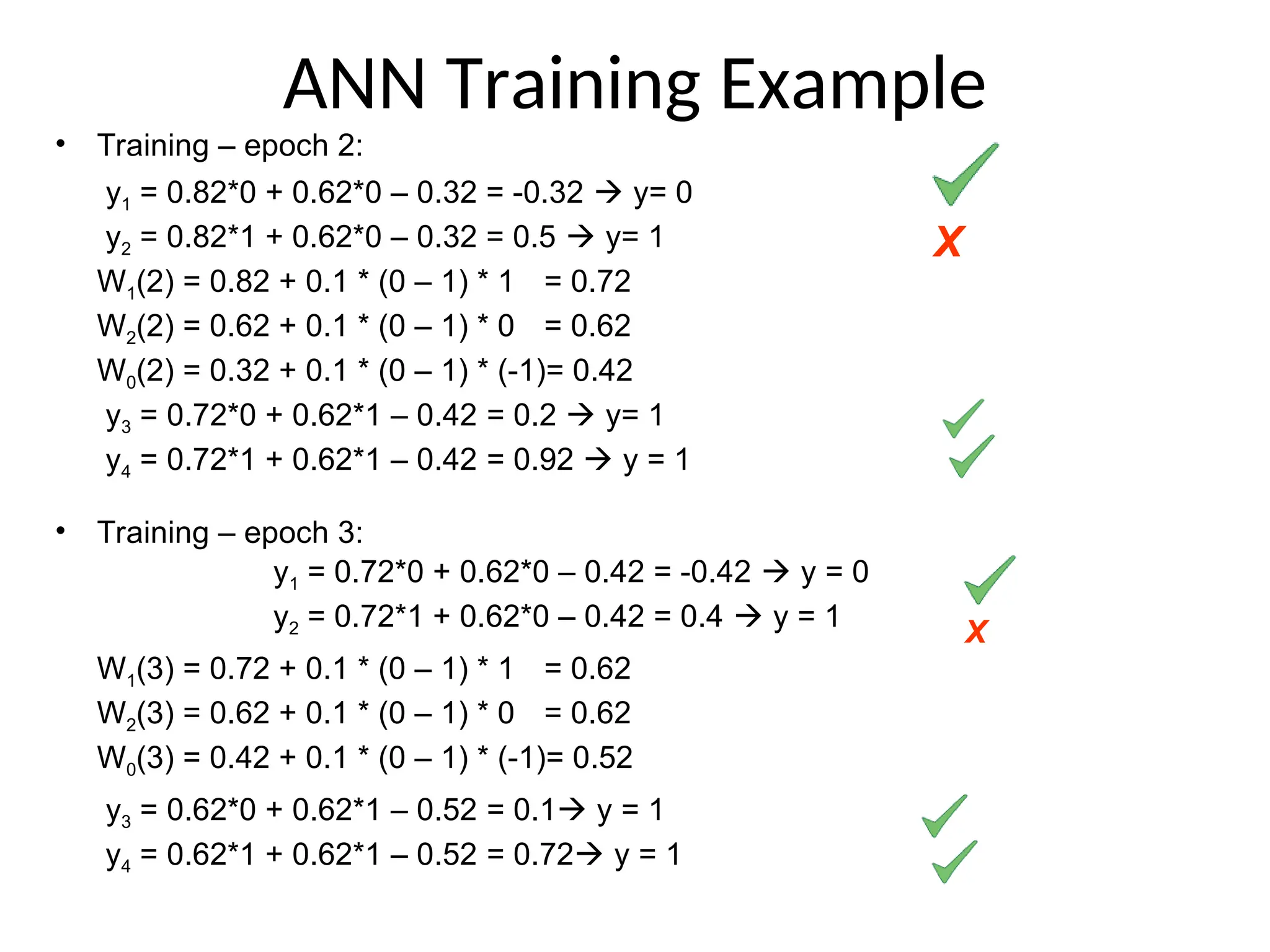
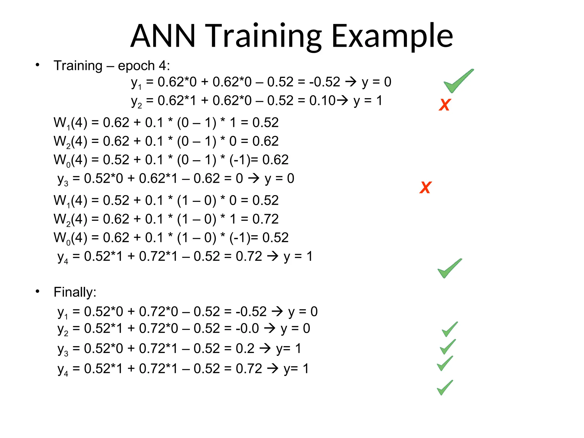
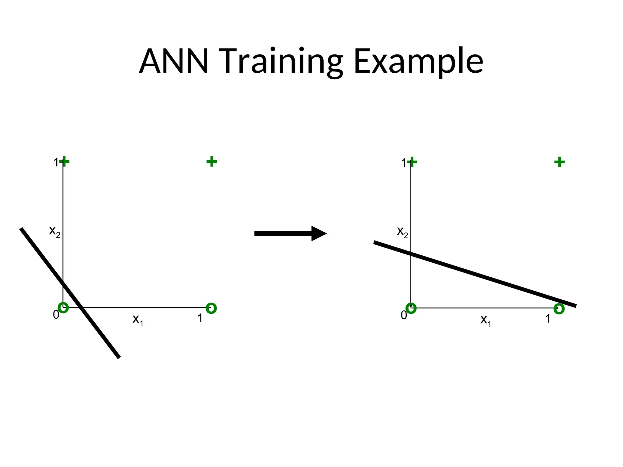
ANN Training Example
• Training – epoch 1:
y1 = 0.92*0 + 0.62*0 – 0.22 = -0.22  y = 0
y2 = 0.92*1 + 0.62*0 – 0.22 = 0.7  y =1
W1(1) = 0.92 + 0.1 * (0 – 1) * 1 = 0.82
W2(1) = 0.62 + 0.1 * (0 – 1) * 0 = 0.62
W0(1) = 0.22 + 0.1 * (0 – 1) * (-1)= 0.32
y3 = 0.82*0 + 0.62*1 – 0.32 = 0.3  y = 1
y4 = 0.82*1 + 0.62*1 – 0.32 = 1.12  y =1
X
Bias 1st
input
(x1)
2nd
input
(x2)
Target
output
-1 0 0 0
-1 1 0 0
-1 0 1 1
-1 1 1 1
Given the following two inputs x1, x2;
find equation that helps to draw the
boundary?
•Let say we have the following initializations:
W1(0) = 0.92, W2(0) = 0.62, W0(0) = 0.22, ή =
0.1

y1 = 0.82*0 + 0.62*0 – 0.32 = -0.32  y= 0
y2 = 0.82*1 + 0.62*0 – 0.32 = 0.5  y= 1
W1(2) = 0.82 + 0.1 * (0 – 1) * 1 = 0.72
W2(2) = 0.62 + 0.1 * (0 – 1) * 0 = 0.62
W0(2) = 0.32 + 0.1 * (0 – 1) * (-1)= 0.42
y3 = 0.72*0 + 0.62*1 – 0.42 = 0.2  y= 1
y4 = 0.72*1 + 0.62*1 – 0.42 = 0.92  y = 1
y1 = 0.72*0 + 0.62*0 – 0.42 = -0.42  y = 0
y2 = 0.72*1 + 0.62*0 – 0.42 = 0.4  y = 1
W1(3) = 0.72 + 0.1 * (0 – 1) * 1 = 0.62
W2(3) = 0.62 + 0.1 * (0 – 1) * 0 = 0.62
W0(3) = 0.42 + 0.1 * (0 – 1) * (-1)= 0.52
y3 = 0.62*0 + 0.62*1 – 0.52 = 0.1 y = 1
y4 = 0.62*1 + 0.62*1 – 0.52 = 0.72 y = 1
X
X

y1 = 0.62*0 + 0.62*0 – 0.52 = -0.52  y = 0
y2 = 0.62*1 + 0.62*0 – 0.52 = 0.10 y = 1
W1(4) = 0.62 + 0.1 * (0 – 1) * 1 = 0.52
W2(4) = 0.62 + 0.1 * (0 – 1) * 0 = 0.62
W0(4) = 0.52 + 0.1 * (0 – 1) * (-1)= 0.62
y3 = 0.52*0 + 0.62*1 – 0.62 = 0  y = 0
W1(4) = 0.52 + 0.1 * (1 – 0) * 0 = 0.52
W2(4) = 0.62 + 0.1 * (1 – 0) * 1 = 0.72
W0(4) = 0.62 + 0.1 * (1 – 0) * (-1)= 0.52
y4 = 0.52*1 + 0.72*1 – 0.52 = 0.72  y = 1
• Finally:
y1 = 0.52*0 + 0.72*0 – 0.52 = -0.52  y = 0
y2 = 0.52*1 + 0.72*0 – 0.52 = -0.0  y = 0
y3 = 0.52*0 + 0.72*1 – 0.52 = 0.2  y= 1
y4 = 0.52*1 + 0.72*1 – 0.52 = 0.72  y= 1
X
X

+ +
1
o 1
0
x2
x1
o
+ +
1
o 1
0
x2
x1
o

Logical Functions
• McCulloch and Pitts: Boolean function can be implemented with a
artificial neuron (not XOR).
W0 = 1.5
W1 = 1
W2 = 1
AND
a1
a2
a0
W0 = 0.5
W1 = 1
W2 = 1
OR
a1
a2
a0
W0 = -0.5
W1 = -1
NOT
a0
a1
A B Output
0 0 0
0 1 0
1 0 0
1 1 1
AND Function
A B Output
0 0 0
0 1 1
1 0 1
1 1 1
OR Function
A Output
0 1
1 0
NOT Function

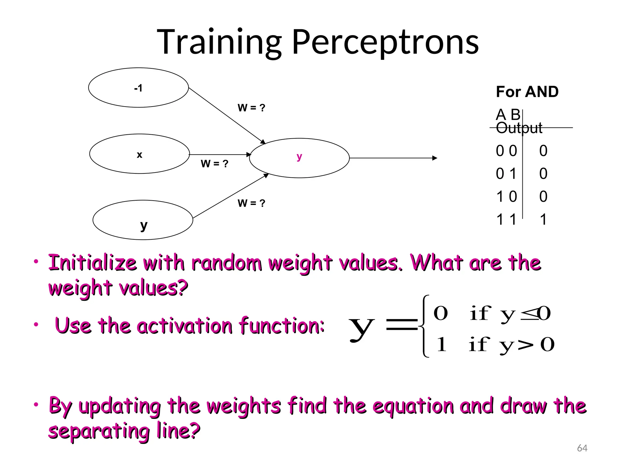
64
Training Perceptrons
y
y
x
-1
W = ?
W = ?
W = ?
For AND
A B
Output
0 0 0
0 1 0
1 0 0
1 1 1
• Initialize with random weight values. What are the
Initialize with random weight values. What are the
weight values?
weight values?
• Use the activation function:
Use the activation function:
• By updating the weights find the equation and draw the
By updating the weights find the equation and draw the
separating line?
separating line?







 0
y
if
1
0
y
if
0
y

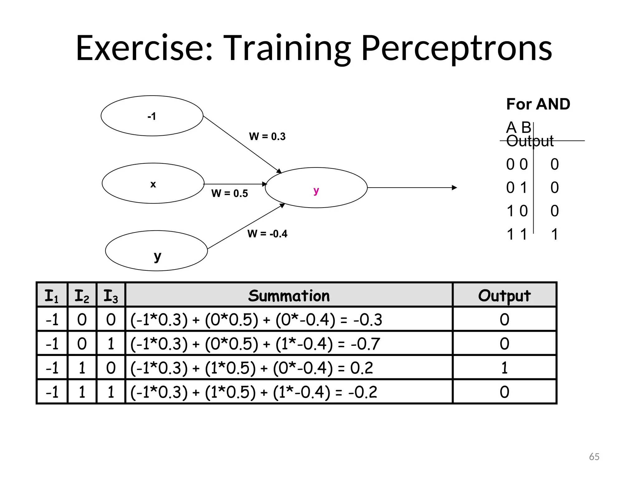
65
Exercise: Training Perceptrons
y
y
x
-1
W = 0.3
W = -0.4
W = 0.5
I1 I2 I3 Summation Output
-1 0 0 (-1*0.3) + (0*0.5) + (0*-0.4) = -0.3 0
-1 0 1 (-1*0.3) + (0*0.5) + (1*-0.4) = -0.7 0
-1 1 0 (-1*0.3) + (1*0.5) + (0*-0.4) = 0.2 1
-1 1 1 (-1*0.3) + (1*0.5) + (1*-0.4) = -0.2 0
For AND
A B
Output
0 0 0
0 1 0
1 0 0
1 1 1

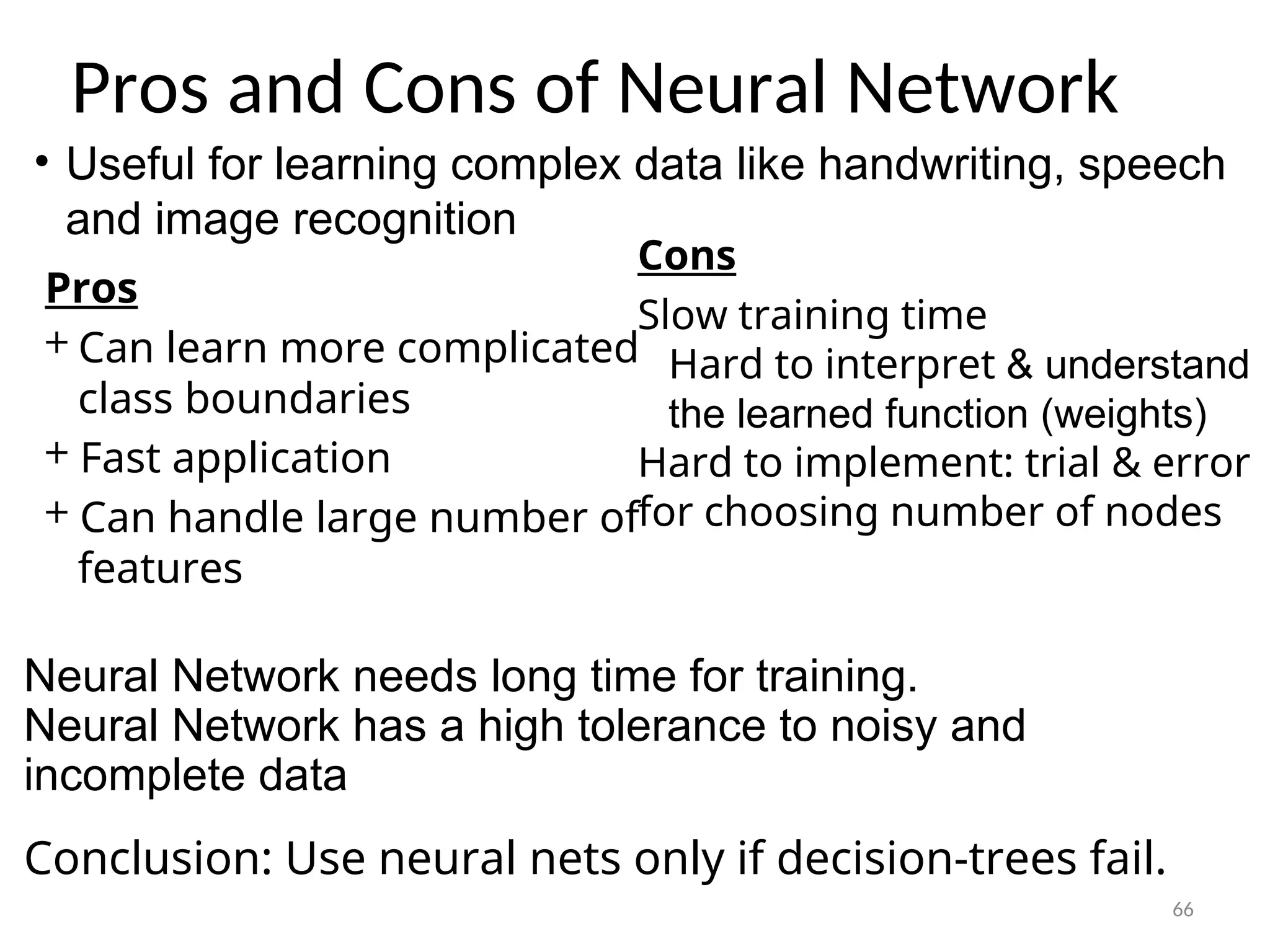
Pros and Cons of Neural Network
Cons

Slow training time
Hard to interpret & understand
the learned function (weights)

Hard to implement: trial & error
for choosing number of nodes
Pros
+ Can learn more complicated
class boundaries
+ Fast application
+ Can handle large number of
features
Neural Network needs long time for training.
Neural Network has a high tolerance to noisy and
incomplete data
Conclusion: Use neural nets only if decision-trees fail.
66
• Useful for learning complex data like handwriting, speech
and image recognition

3 DM Classification HFCS kilometres .ppt

More Related Content

Similar to 3 DM Classification HFCS kilometres .ppt

Recently uploaded

3 DM Classification HFCS kilometres .ppt

Editor's Notes