Clustering
1
Cluster Analysis
 Cluster: a collection of data objects
 Similar to one another within the same cluster
 Dissimilar to the objects in other clusters
 Cluster analysis
 Finding similarities between data according to the characteristics
found in the data and grouping similar data objects into clusters
 Unsupervised learning: no predefined classes
 Typical applications
 As a stand-alone tool to get insight into data distribution
 As a preprocessing step for other algorithms
 For Outlier Analysis
2
Clustering: Rich Applications and
Multidisciplinary Efforts
 Pattern Recognition
 Spatial Data Analysis
 Create thematic maps in GIS by clustering feature spaces
 Detect spatial clusters or for other spatial mining tasks
 Image Processing
 Economic Science (especially market research)
 WWW
 Document classification
 Cluster Weblog data to discover groups of similar access patterns
3
Examples of Clustering Applications
 Marketing: Help marketers discover distinct groups in their customer
bases, and then use this knowledge to develop targeted marketing
programs
 Land use: Identification of areas of similar land use in an earth
observation database
 Insurance: Identifying groups of motor insurance policy holders with a
high average claim cost
 City-planning: Identifying groups of houses according to their house
type, value, and geographical location
 Earth-quake studies: Observed earth quake epicenters should be
clustered along continent faults
4
Clustering Quality
 A good clustering method will produce high quality
clusters with
 high intra-class similarity
 low inter-class similarity
 The quality of a clustering result depends on both the
similarity measure used by the method and its
implementation
5
Measure the Quality of Clustering
 Dissimilarity/Similarity metric: Similarity is expressed in terms of a
distance function, typically metric: d(i, j)
 There is a separate “quality” function that measures the “goodness” of a cluster.
 The definitions of distance functions are usually very different for
interval-scaled, boolean, categorical, ordinal ratio, and vector
variables.
 Weights should be associated with different variables based on
applications and data semantics.
 It is hard to define “similar enough” or “good enough”
 the answer is typically highly subjective.
6
Requirements of Clustering in Data
Mining
 Scalability
 Ability to deal with different types of attributes
 Discovery of clusters with arbitrary shape
 Minimal requirements for domain knowledge to determine input
parameters
 Able to deal with noise and outliers
 Insensitive to order of input records
 High dimensionality
 Incorporation of user-specified constraints
 Interpretability and usability
7
Types of Data
Clustering Data Structures
 Data matrix
 Two modes
 Object by variable structure
 Dissimilarity matrix
 One mode
 Object by object structure
8


















npx...nfx...n1x
...............
ipx...ifx...i1x
...............
1px...1fx...11x
















0...)2,()1,(
:::
)2,3()
...ndnd
0dd(3,1
0d(2,1)
0
Type of data in clustering analysis
 Interval-scaled variables
 Binary variables
 Nominal, ordinal, and ratio variables
 Variables of mixed types
9
Interval-scaled variables
 Continuous measurements
 Standardize data
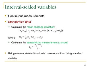
 Calculate the mean absolute deviation:
where
 Calculate the standardized measurement (z-score)
 Using mean absolute deviation is more robust than using standard
deviation
10
.)...
21
1
nffff
xx(xnm +++=
|)|...|||(|1
21 fnffffff
mxmxmxns −++−+−=
f
fif
if s
mx
z
−
=
Similarity and Dissimilarity Between
Objects
 Distances are normally used to measure the similarity or
dissimilarity between two data objects
 Some popular ones include: Minkowski distance
where i = (xi1, xi2, …, xip) and j = (xj1, xj2, …, xjp) are two p-dimensional
data objects, and q is a positive integer
 If q = 1, d is Manhattan distance
11
q
q
pp
qq
j
x
i
x
j
x
i
x
j
x
i
xjid )||...|||(|),(
2211
−++−+−=
||...||||),(
2211 pp j
x
i
x
j
x
i
x
j
x
i
xjid −++−+−=
Similarity and Dissimilarity Between
Objects (Cont.)
 If q = 2, d is Euclidean distance
 Weighted Euclidean distance
 Properties of Euclidean and Manhattan distance
 d(i,j) ≥ 0
 d(i,i) = 0
 d(i,j) = d(j,i)
 d(i,j) ≤ d(i,k) + d(k,j)
12
)||...|||(|),( 22
22
2
11 pp j
x
i
x
j
x
i
x
j
x
i
xjid −++−+−=
Binary Variables
 A contingency table for
binary data
 Distance measure for
symmetric binary variables:
 Distance measure for
asymmetric binary variables:
 Jaccard coefficient (similarity
measure for asymmetric
binary variables):
13
dcba
cbjid
+++
+=),(
cba
cbjid
++
+=),(
pdbcasum
dcdc
baba
sum
++
+
+
0
1
01
Object i
Object j
),(1),( jidjisim −=
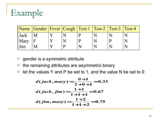
Example
 gender is a symmetric attribute
 the remaining attributes are asymmetric binary
 let the values Y and P be set to 1, and the value N be set to 0
14
Name Gender Fever Cough Test-1 Test-2 Test-3 Test-4
Jack M Y N P N N N
Mary F Y N P N P N
Jim M Y P N N N N
75.0
211
21
),(
67.0
111
11
),(
33.0
102
10
),(
=
++
+
=
=
++
+
=
=
++
+
=
maryjimd
jimjackd
maryjackd
Categorical or Nominal Variables
 A generalization of the binary variable in that it can take
more than 2 states, e.g., red, yellow, blue, green
 Method 1: Simple matching
 m: # of matches, p: total # of variables
 Method 2: use a large number of binary variables
 creating a new binary variable for each of the M nominal states
 Using similarity measures of binary variables
15
p
mpjid −=),(
Ordinal Variables
 An ordinal variable can be discrete or continuous
 Order is important, e.g., rank
 Can be treated like interval-scaled
 replace xif by their rank
 map the range of each variable onto [0, 1] by replacing i-th object in
the f-th variable by
 compute the dissimilarity using methods for interval-scaled
variables
16
1
1
−
−
=
f
if
if M
r
z
},...,1{ fif
Mr ∈
Ratio-Scaled Variables
 Ratio-scaled variable: a positive measurement on a
nonlinear scale, approximately at exponential scale, such
as AeBt
or Ae-Bt
 Methods:
 treat them like interval-scaled variables—not a good choice
 apply logarithmic transformation
yif = log(xif)
 treat them as continuous ordinal data treat their rank as interval-
scaled
17
Variables of Mixed Types
 A database may contain all the six types of variables
 symmetric binary, asymmetric binary, nominal, ordinal, interval
and ratio
 One may use a weighted formula to combine their
effects
 f is binary or nominal:
dij
(f)
= 0 if xif = xjf , or dij
(f)
= 1 otherwise
 f is interval-based: use the normalized distance
 f is ordinal or ratio-scaled
 compute ranks rif and
 and treat zif as interval-scaled
18
)(
1
)()(
1
),( f
ij
p
f
f
ij
f
ij
p
f
d
jid
δ
δ
=
=
Σ
Σ
=
1
1
−
−
=
f
if
M
rzif
Vector Objects
 Cosine measure
s(x,y) = xt
. y / ||x|| ||y||
xt
. y = number of attributes shared by x and y
 Tanimoto distance
s(x,y) = xt
. y / xt
. x + yt
. y - xt
. y
Ratio of attributes shared by x and y to number of
attributes possessed by x or y
19
22
2
2
1 ...|||| pxxxx +++=

3.1 clustering

  • 1.
  • 2.
    Cluster Analysis  Cluster:a collection of data objects  Similar to one another within the same cluster  Dissimilar to the objects in other clusters  Cluster analysis  Finding similarities between data according to the characteristics found in the data and grouping similar data objects into clusters  Unsupervised learning: no predefined classes  Typical applications  As a stand-alone tool to get insight into data distribution  As a preprocessing step for other algorithms  For Outlier Analysis 2
  • 3.
    Clustering: Rich Applicationsand Multidisciplinary Efforts  Pattern Recognition  Spatial Data Analysis  Create thematic maps in GIS by clustering feature spaces  Detect spatial clusters or for other spatial mining tasks  Image Processing  Economic Science (especially market research)  WWW  Document classification  Cluster Weblog data to discover groups of similar access patterns 3
  • 4.
    Examples of ClusteringApplications  Marketing: Help marketers discover distinct groups in their customer bases, and then use this knowledge to develop targeted marketing programs  Land use: Identification of areas of similar land use in an earth observation database  Insurance: Identifying groups of motor insurance policy holders with a high average claim cost  City-planning: Identifying groups of houses according to their house type, value, and geographical location  Earth-quake studies: Observed earth quake epicenters should be clustered along continent faults 4
  • 5.
    Clustering Quality  Agood clustering method will produce high quality clusters with  high intra-class similarity  low inter-class similarity  The quality of a clustering result depends on both the similarity measure used by the method and its implementation 5
  • 6.
    Measure the Qualityof Clustering  Dissimilarity/Similarity metric: Similarity is expressed in terms of a distance function, typically metric: d(i, j)  There is a separate “quality” function that measures the “goodness” of a cluster.  The definitions of distance functions are usually very different for interval-scaled, boolean, categorical, ordinal ratio, and vector variables.  Weights should be associated with different variables based on applications and data semantics.  It is hard to define “similar enough” or “good enough”  the answer is typically highly subjective. 6
  • 7.
    Requirements of Clusteringin Data Mining  Scalability  Ability to deal with different types of attributes  Discovery of clusters with arbitrary shape  Minimal requirements for domain knowledge to determine input parameters  Able to deal with noise and outliers  Insensitive to order of input records  High dimensionality  Incorporation of user-specified constraints  Interpretability and usability 7
  • 8.
    Types of Data ClusteringData Structures  Data matrix  Two modes  Object by variable structure  Dissimilarity matrix  One mode  Object by object structure 8                   npx...nfx...n1x ............... ipx...ifx...i1x ............... 1px...1fx...11x                 0...)2,()1,( ::: )2,3() ...ndnd 0dd(3,1 0d(2,1) 0
  • 9.
    Type of datain clustering analysis  Interval-scaled variables  Binary variables  Nominal, ordinal, and ratio variables  Variables of mixed types 9
  • 10.
    Interval-scaled variables  Continuousmeasurements  Standardize data  Calculate the mean absolute deviation: where  Calculate the standardized measurement (z-score)  Using mean absolute deviation is more robust than using standard deviation 10 .)... 21 1 nffff xx(xnm +++= |)|...|||(|1 21 fnffffff mxmxmxns −++−+−= f fif if s mx z − =
  • 11.
    Similarity and DissimilarityBetween Objects  Distances are normally used to measure the similarity or dissimilarity between two data objects  Some popular ones include: Minkowski distance where i = (xi1, xi2, …, xip) and j = (xj1, xj2, …, xjp) are two p-dimensional data objects, and q is a positive integer  If q = 1, d is Manhattan distance 11 q q pp qq j x i x j x i x j x i xjid )||...|||(|),( 2211 −++−+−= ||...||||),( 2211 pp j x i x j x i x j x i xjid −++−+−=
  • 12.
    Similarity and DissimilarityBetween Objects (Cont.)  If q = 2, d is Euclidean distance  Weighted Euclidean distance  Properties of Euclidean and Manhattan distance  d(i,j) ≥ 0  d(i,i) = 0  d(i,j) = d(j,i)  d(i,j) ≤ d(i,k) + d(k,j) 12 )||...|||(|),( 22 22 2 11 pp j x i x j x i x j x i xjid −++−+−=
  • 13.
    Binary Variables  Acontingency table for binary data  Distance measure for symmetric binary variables:  Distance measure for asymmetric binary variables:  Jaccard coefficient (similarity measure for asymmetric binary variables): 13 dcba cbjid +++ +=),( cba cbjid ++ +=),( pdbcasum dcdc baba sum ++ + + 0 1 01 Object i Object j ),(1),( jidjisim −=
  • 14.
    Example  gender isa symmetric attribute  the remaining attributes are asymmetric binary  let the values Y and P be set to 1, and the value N be set to 0 14 Name Gender Fever Cough Test-1 Test-2 Test-3 Test-4 Jack M Y N P N N N Mary F Y N P N P N Jim M Y P N N N N 75.0 211 21 ),( 67.0 111 11 ),( 33.0 102 10 ),( = ++ + = = ++ + = = ++ + = maryjimd jimjackd maryjackd
  • 15.
    Categorical or NominalVariables  A generalization of the binary variable in that it can take more than 2 states, e.g., red, yellow, blue, green  Method 1: Simple matching  m: # of matches, p: total # of variables  Method 2: use a large number of binary variables  creating a new binary variable for each of the M nominal states  Using similarity measures of binary variables 15 p mpjid −=),(
  • 16.
    Ordinal Variables  Anordinal variable can be discrete or continuous  Order is important, e.g., rank  Can be treated like interval-scaled  replace xif by their rank  map the range of each variable onto [0, 1] by replacing i-th object in the f-th variable by  compute the dissimilarity using methods for interval-scaled variables 16 1 1 − − = f if if M r z },...,1{ fif Mr ∈
  • 17.
    Ratio-Scaled Variables  Ratio-scaledvariable: a positive measurement on a nonlinear scale, approximately at exponential scale, such as AeBt or Ae-Bt  Methods:  treat them like interval-scaled variables—not a good choice  apply logarithmic transformation yif = log(xif)  treat them as continuous ordinal data treat their rank as interval- scaled 17
  • 18.
    Variables of MixedTypes  A database may contain all the six types of variables  symmetric binary, asymmetric binary, nominal, ordinal, interval and ratio  One may use a weighted formula to combine their effects  f is binary or nominal: dij (f) = 0 if xif = xjf , or dij (f) = 1 otherwise  f is interval-based: use the normalized distance  f is ordinal or ratio-scaled  compute ranks rif and  and treat zif as interval-scaled 18 )( 1 )()( 1 ),( f ij p f f ij f ij p f d jid δ δ = = Σ Σ = 1 1 − − = f if M rzif
  • 19.
    Vector Objects  Cosinemeasure s(x,y) = xt . y / ||x|| ||y|| xt . y = number of attributes shared by x and y  Tanimoto distance s(x,y) = xt . y / xt . x + yt . y - xt . y Ratio of attributes shared by x and y to number of attributes possessed by x or y 19 22 2 2 1 ...|||| pxxxx +++=