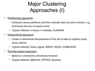
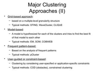
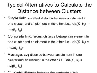
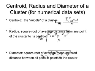
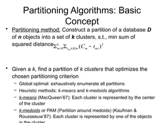
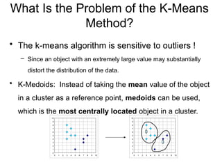
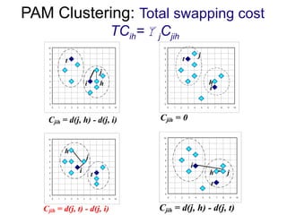
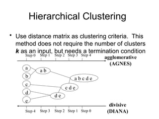
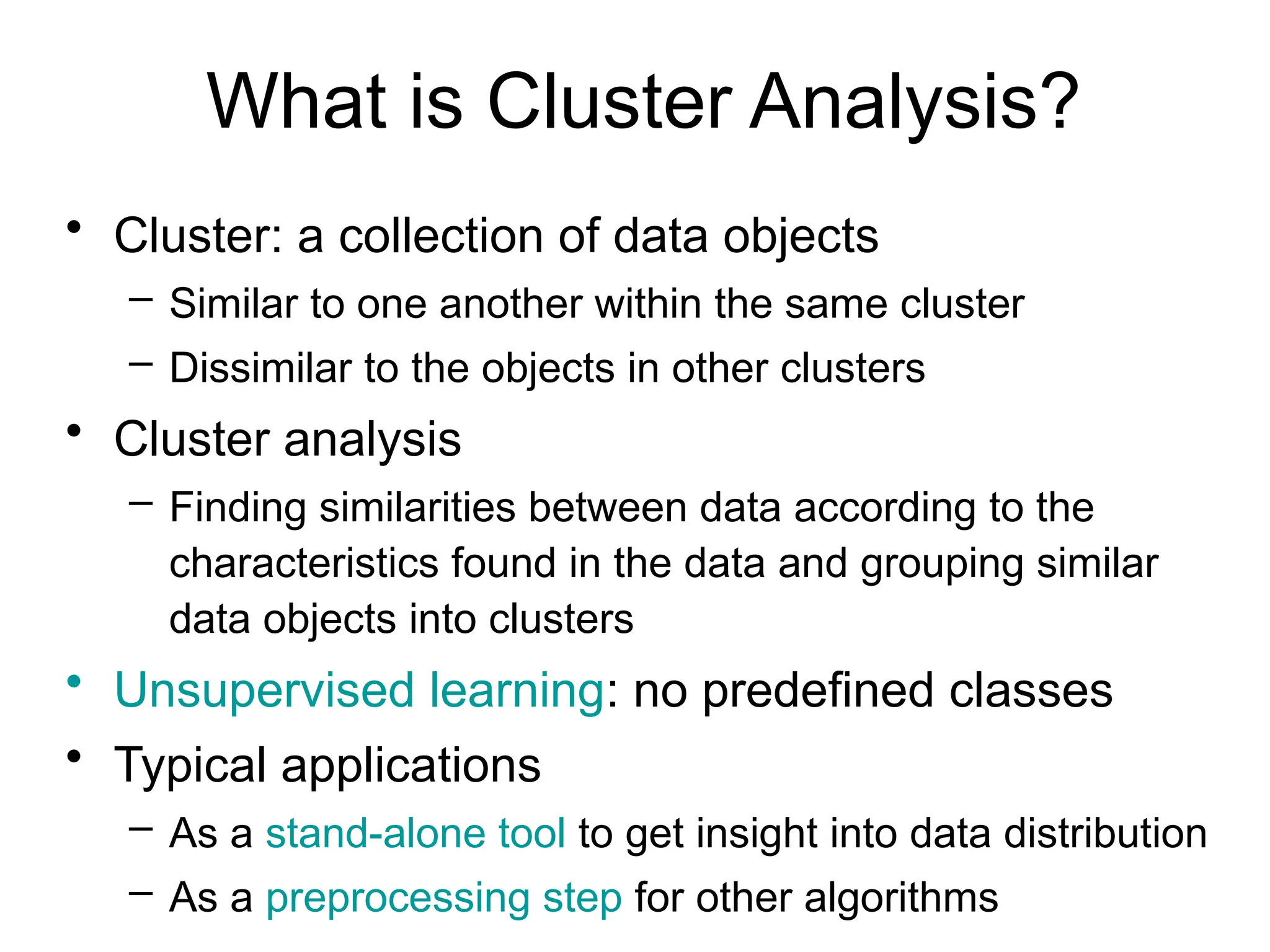
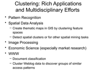
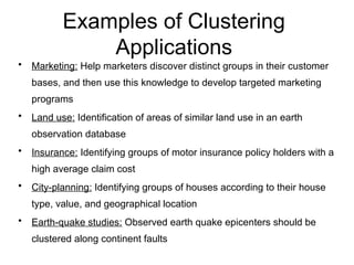
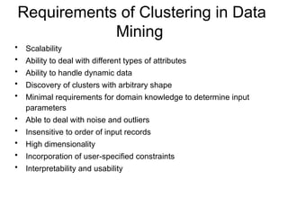
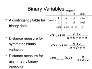
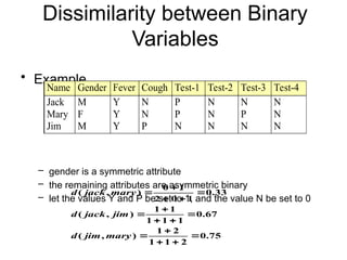
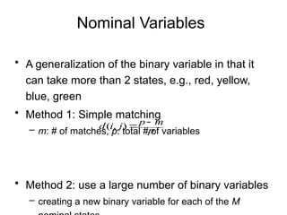
What is Cluster Analysis?
• Cluster: a collection of data objects
– Similar to one another within the same cluster
– Dissimilar to the objects in other clusters
• Cluster analysis
– Finding similarities between data according to the
characteristics found in the data and grouping similar
data objects into clusters
• Unsupervised learning: no predefined classes
• Typical applications
– As a stand-alone tool to get insight into data distribution
– As a preprocessing step for other algorithms
Clustering: Rich Applications
and Multidisciplinary Efforts
• Pattern Recognition
• Spatial Data Analysis
– Create thematic maps in GIS by clustering feature
spaces
– Detect spatial clusters or for other spatial mining tasks
• Image Processing
• Economic Science (especially market research)
• WWW
– Document classification
– Cluster Weblog data to discover groups of similar
access patterns
Examples of Clustering
Applications
• Marketing: Help marketers discover distinct groups in their customer
bases, and then use this knowledge to develop targeted marketing
programs
• Land use: Identification of areas of similar land use in an earth
observation database
• Insurance: Identifying groups of motor insurance policy holders with a
high average claim cost
• City-planning: Identifying groups of houses according to their house
type, value, and geographical location
• Earth-quake studies: Observed earth quake epicenters should be
clustered along continent faults
Quality: What Is Good
Clustering?
• A good clustering method will produce high
quality clusters with
– high intra-class similarity
– low inter-class similarity
• The quality of a clustering result depends on
both the similarity measure used by the method
and its implementation
• The quality of a clustering method is also
measured by its ability to discover some or all of
Measure the Quality of
Clustering
• Dissimilarity/Similarity metric: Similarity is
expressed in terms of a distance function,
typically metric: d(i, j)
• There is a separate “quality” function that
measures the “goodness” of a cluster.
• The definitions of distance functions are usually
very different for interval-scaled, boolean,
categorical, ordinal ratio, and vector variables.
• Weights should be associated with different
variables based on applications and data
semantics.
Requirements of Clustering in Data
Mining
• Scalability
• Ability to deal with different types of attributes
• Ability to handle dynamic data
• Discovery of clusters with arbitrary shape
• Minimal requirements for domain knowledge to determine input
parameters
• Able to deal with noise and outliers
• Insensitive to order of input records
• High dimensionality
• Incorporation of user-specified constraints
• Interpretability and usability
Data Structures
• Data matrix
– (two modes)
• Dissimilarity matrix
– (one mode)


















np
x
...
nf
x
...
n1
x
...
...
...
...
...
ip
x
...
if
x
...
i1
x
...
...
...
...
...
1p
x
...
1f
x
...
11
x
















0
...
)
2
,
(
)
1
,
(
:
:
:
)
2
,
3
(
)
...
n
d
n
d
0
d
d(3,1
0
d(2,1)
0
Type of data in clustering
analysis
• Interval-scaled variables
• Binary variables
• Nominal, ordinal, and ratio variables
• Variables of mixed types
Interval-valued variables
• Standardize data
– Calculate the mean absolute deviation:
where
– Calculate the standardized measurement (z-score)
• Using mean absolute deviation is more robust
than using standard deviation
.
)
...
2
1
1
nf
f
f
f
x
x
(x
n
m 



|)
|
...
|
|
|
(|
1
2
1 f
nf
f
f
f
f
f
m
x
m
x
m
x
n
s 






f
f
if
if s
m
x
z


Similarity and Dissimilarity
Between Objects
• Distances are normally used to measure the
similarity or dissimilarity between two data
objects
• Some popular ones include: Minkowski
distance:
where i = (xi1, xi2, …, xip) and j = (xj1, xj2, …, xjp) are two
p-dimensional data objects, and q is a positive
integer
q
q
p
p
q
q
j
x
i
x
j
x
i
x
j
x
i
x
j
i
d )
|
|
...
|
|
|
(|
)
,
(
2
2
1
1







|
|
...
|
|
|
|
)
,
(
2
2
1
1 p
p j
x
i
x
j
x
i
x
j
x
i
x
j
i
d 






Similarity and Dissimilarity
Between Objects (Cont.)
• If q = 2, d is Euclidean distance:
– Properties
• d(i,j)  0
• d(i,i) = 0
• d(i,j) = d(j,i)
• d(i,j)  d(i,k) + d(k,j)
• Also, one can use weighted distance,
parametric Pearson product moment
correlation, or other disimilarity measures
)
|
|
...
|
|
|
(|
)
,
( 2
2
2
2
2
1
1 p
p j
x
i
x
j
x
i
x
j
x
i
x
j
i
d 






Binary Variables
• A contingency table for
binary data
• Distance measure for
symmetric binary
variables:
• Distance measure for
asymmetric binary
variables:
d
c
b
a
c
b
j
i
d





)
,
(
c
b
a
c
b
j
i
d




)
,
(
p
d
b
c
a
sum
d
c
d
c
b
a
b
a
sum




0
1
0
1
Object i
Object j
c
b
a
a
j
i
simJaccard



)
,
(
Dissimilarity between Binary
Variables
• Example
– gender is a symmetric attribute
– the remaining attributes are asymmetric binary
– let the values Y and P be set to 1, and the value N be set to 0
Name Gender Fever Cough Test-1 Test-2 Test-3 Test-4
Jack M Y N P N N N
Mary F Y N P N P N
Jim M Y P N N N N
75
.
0
2
1
1
2
1
)
,
(
67
.
0
1
1
1
1
1
)
,
(
33
.
0
1
0
2
1
0
)
,
(















mary
jim
d
jim
jack
d
mary
jack
d
Nominal Variables
• A generalization of the binary variable in that it
can take more than 2 states, e.g., red, yellow,
blue, green
• Method 1: Simple matching
– m: # of matches, p: total # of variables
• Method 2: use a large number of binary variables
– creating a new binary variable for each of the M
p
m
p
j
i
d 

)
,
(
Ordinal Variables
• An ordinal variable can be discrete or continuous
• Order is important, e.g., rank
• Can be treated like interval-scaled
– replace xif by their rank
– map the range of each variable onto [0, 1] by replacing
i-th object in the f-th variable by
– compute the dissimilarity using methods for interval-
scaled variables
1
1



f
if
if M
r
z
}
,...,
1
{ f
if
M
r 
Ratio-Scaled Variables
• Ratio-scaled variable: a positive measurement on
a nonlinear scale, approximately at exponential
scale, such as AeBt
or Ae-Bt
• Methods:
– treat them like interval-scaled variables—not a good
choice! (why?—the scale can be distorted)
– apply logarithmic transformation
yif = log(xif)
– treat them as continuous ordinal data treat their rank as
interval-scaled
Variables of Mixed Types
• A database may contain all the six types of
variables
– symmetric binary, asymmetric binary, nominal,
ordinal, interval and ratio
• One may use a weighted formula to combine
their effects
– f is binary or nominal:
dij
(f)
= 0 if xif = xjf , or dij
(f)
= 1 otherwise
– f is interval-based: use the normalized distance
– f is ordinal or ratio-scaled
• compute ranks rif and
)
(
1
)
(
)
(
1
)
,
( f
ij
p
f
f
ij
f
ij
p
f
d
j
i
d







1
1



f
if
M
r
zif
Vector Objects
• Vector objects: keywords in documents,
gene features in micro-arrays, etc.
• Broad applications: information retrieval,
biologic taxonomy, etc.
• Cosine measure
• A variant: Tanimoto coefficient
Major Clustering
Approaches (I)
• Partitioning approach:
– Construct various partitions and then evaluate them by some criterion, e.g.,
minimizing the sum of square errors
– Typical methods: k-means, k-medoids, CLARANS
• Hierarchical approach:
– Create a hierarchical decomposition of the set of data (or objects) using
some criterion
– Typical methods: Diana, Agnes, BIRCH, ROCK, CAMELEON
• Density-based approach:
– Based on connectivity and density functions
– Typical methods: DBSACN, OPTICS, DenClue
Major Clustering
Approaches (II)
• Grid-based approach:
– based on a multiple-level granularity structure
– Typical methods: STING, WaveCluster, CLIQUE
• Model-based:
– A model is hypothesized for each of the clusters and tries to find the best fit
of that model to each other
– Typical methods: EM, SOM, COBWEB
• Frequent pattern-based:
– Based on the analysis of frequent patterns
– Typical methods: pCluster
• User-guided or constraint-based:
– Clustering by considering user-specified or application-specific constraints
– Typical methods: COD (obstacles), constrained clustering
Typical Alternatives to Calculate the
Distance between Clusters
• Single link: smallest distance between an element in
one cluster and an element in the other, i.e., dis(Ki, Kj) =
min(tip, tjq)
• Complete link: largest distance between an element in
one cluster and an element in the other, i.e., dis(Ki, Kj) =
max(tip, tjq)
• Average: avg distance between an element in one
cluster and an element in the other, i.e., dis(Ki, Kj) =
avg(tip, tjq)
Centroid, Radius and Diameter of a
Cluster (for numerical data sets)
• Centroid: the “middle” of a cluster
• Radius: square root of average distance from any point
of the cluster to its centroid
• Diameter: square root of average mean squared
distance between all pairs of points in the cluster
N
t
N
i ip
m
C
)
(
1



N
m
c
ip
t
N
i
m
R
2
)
(
1




)
1
(
2
)
(
1
1







N
N
iq
t
ip
t
N
i
N
i
m
D
Partitioning Algorithms: Basic
Concept
• Partitioning method: Construct a partition of a database D
of n objects into a set of k clusters, s.t., min sum of
squared distance
• Given a k, find a partition of k clusters that optimizes the
chosen partitioning criterion
– Global optimal: exhaustively enumerate all partitions
– Heuristic methods: k-means and k-medoids algorithms
– k-means (MacQueen’67): Each cluster is represented by the center
of the cluster
– k-medoids or PAM (Partition around medoids) (Kaufman &
Rousseeuw’87): Each cluster is represented by one of the objects
2
1 )
( mi
m
Km
t
k
m t
C
mi


 

The K-Means Clustering Method
• Given k, the k-means algorithm is
implemented in four steps:
– Partition objects into k nonempty subsets
– Compute seed points as the centroids of the
clusters of the current partition (the centroid is the
center, i.e., mean point, of the cluster)
– Assign each object to the cluster with the nearest
seed point
– Go back to Step 2, stop when no more new
assignment
The K-Means Clustering Method
• Example
0
1
2
3
4
5
6
7
8
9
10
0 1 2 3 4 5 6 7 8 9 10
0
1
2
3
4
5
6
7
8
9
10
0 1 2 3 4 5 6 7 8 9 10
0
1
2
3
4
5
6
7
8
9
10
0 1 2 3 4 5 6 7 8 9 10
0
1
2
3
4
5
6
7
8
9
10
0 1 2 3 4 5 6 7 8 9 10
0
1
2
3
4
5
6
7
8
9
10
0 1 2 3 4 5 6 7 8 9 10
K=2
Arbitrarily choose K
object as initial
cluster center
Assign
each
objects
to most
similar
center
Update
the
cluster
means
Update
the
cluster
means
reassign
reassign
Comments on the K-Means
Method
• Strength: Relatively efficient: O(tkn), where n is # objects, k
is # clusters, and t is # iterations. Normally, k, t << n.
• Comparing: PAM: O(k(n-k)2
), CLARA: O(ks2
+ k(n-k))
• Comment: Often terminates at a local optimum. The global
optimum may be found using techniques such as:
deterministic annealing and genetic algorithms
• Weakness
– Applicable only when mean is defined, then what about categorical
data?
– Need to specify k, the number of clusters, in advance
– Unable to handle noisy data and outliers
– Not suitable to discover clusters with non-convex shapes
Variations of the K-Means Method
• A few variants of the k-means which differ in
– Selection of the initial k means
– Dissimilarity calculations
– Strategies to calculate cluster means
• Handling categorical data: k-modes (Huang’98)
– Replacing means of clusters with modes
– Using new dissimilarity measures to deal with categorical objects
– Using a frequency-based method to update modes of clusters
– A mixture of categorical and numerical data: k-prototype method
What Is the Problem of the K-Means
Method?
• The k-means algorithm is sensitive to outliers !
– Since an object with an extremely large value may substantially
distort the distribution of the data.
• K-Medoids: Instead of taking the mean value of the object
in a cluster as a reference point, medoids can be used,
which is the most centrally located object in a cluster.
0
1
2
3
4
5
6
7
8
9
10
0 1 2 3 4 5 6 7 8 9 10
0
1
2
3
4
5
6
7
8
9
10
0 1 2 3 4 5 6 7 8 9 10
The K-Medoids Clustering Method
• Find representative objects, called medoids, in clusters
• PAM (Partitioning Around Medoids, 1987)
– starts from an initial set of medoids and iteratively replaces one
of the medoids by one of the non-medoids if it improves the total
distance of the resulting clustering
– PAM works effectively for small data sets, but does not scale
well for large data sets
• CLARA (Kaufmann & Rousseeuw, 1990)
• CLARANS (Ng & Han, 1994): Randomized sampling
• Focusing + spatial data structure (Ester et al., 1995)
A Typical K-Medoids Algorithm (PAM)
0
1
2
3
4
5
6
7
8
9
10
0 1 2 3 4 5 6 7 8 9 10
Total Cost = 20
0
1
2
3
4
5
6
7
8
9
10
0 1 2 3 4 5 6 7 8 9 10
K=2
Arbitrar
y choose
k object
as initial
medoids
0
1
2
3
4
5
6
7
8
9
10
0 1 2 3 4 5 6 7 8 9 10
Assign
each
remaini
ng
object to
nearest
medoids
Randomly select a
nonmedoid
object,Oramdom
Compute
total cost
of
swapping
0
1
2
3
4
5
6
7
8
9
10
0 1 2 3 4 5 6 7 8 9 10
Total Cost = 26
Swapping O
and Oramdom
If quality is
improved.
Do loop
Until no
change
0
1
2
3
4
5
6
7
8
9
10
0 1 2 3 4 5 6 7 8 9 10
PAM (Partitioning Around Medoids)
(1987)
• PAM (Kaufman and Rousseeuw, 1987), built in
Splus
• Use real object to represent the cluster
– Select k representative objects arbitrarily
– For each pair of non-selected object h and selected
object i, calculate the total swapping cost TCih
– For each pair of i and h,
• If TCih < 0, i is replaced by h
• Then assign each non-selected object to the most
similar representative object
PAM Clustering: Total swapping cost
TCih=jCjih
0
1
2
3
4
5
6
7
8
9
10
0 1 2 3 4 5 6 7 8 9 10
j
i
h
t
Cjih = 0
0
1
2
3
4
5
6
7
8
9
10
0 1 2 3 4 5 6 7 8 9 10
t
i h
j
Cjih = d(j, h) - d(j, i)
0
1
2
3
4
5
6
7
8
9
10
0 1 2 3 4 5 6 7 8 9 10
h
i
t
j
Cjih = d(j, t) - d(j, i)
0
1
2
3
4
5
6
7
8
9
10
0 1 2 3 4 5 6 7 8 9 10
t
i
h j
Cjih = d(j, h) - d(j, t)
What Is the Problem with
PAM?
• Pam is more robust than k-means in the
presence of noise and outliers because a
medoid is less influenced by outliers or other
extreme values than a mean
• Pam works efficiently for small data sets but
does not scale well for large data sets.
– O(k(n-k)2
) for each iteration
where n is # of data,k is # of clusters
Sampling based method,
CLARA (Clustering Large
Applications) (1990)
• CLARA (Kaufmann and Rousseeuw in 1990)
– Built in statistical analysis packages, such as S+
• It draws multiple samples of the data set,
applies PAM on each sample, and gives the
best clustering as the output
• Strength: deals with larger data sets than PAM
• Weakness:
– Efficiency depends on the sample size
– A good clustering based on samples will not
CLARANS (“Randomized” CLARA)
(1994)
• CLARANS (A Clustering Algorithm based on
Randomized Search) (Ng and Han’94)
• CLARANS draws sample of neighbors
dynamically
• The clustering process can be presented as
searching a graph where every node is a potential
solution, that is, a set of k medoids
• If the local optimum is found, CLARANS starts
with new randomly selected node in search for a
new local optimum
Hierarchical Clustering
• Use distance matrix as clustering criteria. This
method does not require the number of clusters
k as an input, but needs a termination condition
Step 0 Step 1 Step 2 Step 3 Step 4
b
d
c
e
a a b
d e
c d e
a b c d e
Step 4 Step 3 Step 2 Step 1 Step 0
agglomerative
(AGNES)
divisive
(DIANA)
AGNES (Agglomerative
Nesting)
• Introduced in Kaufmann and Rousseeuw (1990)
• Implemented in statistical analysis packages, e.g.,
Splus
• Use the Single-Link method and the dissimilarity
matrix.
• Merge nodes that have the least dissimilarity
• Go on in a non-descending fashion
• Eventually all nodes belong to the same cluster
0
1
2
3
4
5
6
7
8
9
10
0 1 2 3 4 5 6 7 8 9 10
0
1
2
3
4
5
6
7
8
9
10
0 1 2 3 4 5 6 7 8 9 10
0
1
2
3
4
5
6
7
8
9
10
0 1 2 3 4 5 6 7 8 9 10
Dendrogram: Shows How the Clusters are Merged
Decompose data objects into a several levels of nested
partitioning (tree of clusters), called a dendrogram.
A clustering of the data objects is obtained by cutting the
dendrogram at the desired level, then each connected
component forms a cluster.
DIANA (Divisive Analysis)
• Introduced in Kaufmann and Rousseeuw (1990)
• Implemented in statistical analysis packages,
e.g., Splus
• Inverse order of AGNES
• Eventually each node forms a cluster on its own
0
1
2
3
4
5
6
7
8
9
10
0 1 2 3 4 5 6 7 8 9 10
0
1
2
3
4
5
6
7
8
9
10
0 1 2 3 4 5 6 7 8 9 10
0
1
2
3
4
5
6
7
8
9
10
0 1 2 3 4 5 6 7 8 9 10
Recent Hierarchical Clustering
Methods
• Major weakness of agglomerative clustering
methods
– do not scale well: time complexity of at least O(n2
),
where n is the number of total objects
– can never undo what was done previously
• Integration of hierarchical with distance-based
clustering
– BIRCH (1996): uses CF-tree and incrementally adjusts
the quality of sub-clusters
– ROCK (1999): clustering categorical data by neighbor
and link analysis
Clustering High-Dimensional
Data
• Clustering high-dimensional data
– Many applications: text documents, DNA micro-array data
– Major challenges:
• Many irrelevant dimensions may mask clusters
• Distance measure becomes meaningless—due to equi-distance
• Clusters may exist only in some subspaces
• Methods
– Feature transformation: only effective if most dimensions are relevant
• PCA & SVD useful only when features are highly correlated/redundant
– Feature selection: wrapper or filter approaches
• useful to find a subspace where the data have nice clusters
– Subspace-clustering: find clusters in all the possible subspaces
• CLIQUE, ProClus, and frequent pattern-based clustering
The Curse of Dimensionality
(graphs adapted from Parsons et al. KDD
Explorations 2004)
• Data in only one dimension is
relatively packed
• Adding a dimension “stretch” the
points across that dimension,
making them further apart
• Adding more dimensions will
make the points further apart—
high dimensional data is
extremely sparse
• Distance measure becomes
Why Subspace
Clustering?
(adapted from Parsons et al. SIGKDD
Explorations 2004)
• Clusters may exist only in some subspaces
• Subspace-clustering: find clusters in all the
subspaces
What Is Outlier Discovery?
• What are outliers?
– The set of objects are considerably dissimilar from the
remainder of the data
– Example: Sports: Michael Jordon, Wayne Gretzky, ...
• Problem: Define and find outliers in large data
sets
• Applications:
– Credit card fraud detection
– Telecom fraud detection
– Customer segmentation
– Medical analysis
Outlier Discovery:
Statistical
Approaches
 Assume a model underlying distribution that
generates data set (e.g. normal distribution)
• Use discordancy tests depending on
– data distribution
– distribution parameter (e.g., mean, variance)
– number of expected outliers
• Drawbacks
– most tests are for single attribute
– In many cases, data distribution may not be known
Outlier Discovery: Distance-Based
Approach
• Introduced to counter the main limitations
imposed by statistical methods
– We need multi-dimensional analysis without knowing
data distribution
• Distance-based outlier: A DB(p, D)-outlier is an
object O in a dataset T such that at least a
fraction p of the objects in T lies at a distance
greater than D from O
• Algorithms for mining distance-based outliers
– Index-based algorithm
– Nested-loop algorithm
Density-Based
Local Outlier
Detection
• Distance-based outlier
detection is based on
global distance distribution
• It encounters difficulties to
identify outliers if data is
not uniformly distributed
• Ex. C1 contains 400 loosely
distributed points, C2 has
100 tightly condensed
points, 2 outlier points o1,
o2
• Distance-based method
• Local outlier factor
(LOF)
– Assume outlier is not
crisp
– Each point has a LOF
Summary
• Cluster analysis groups objects based on their
similarity and has wide applications
• Measure of similarity can be computed for
various types of data
• Clustering algorithms can be categorized into
partitioning methods, hierarchical methods,
density-based methods, grid-based methods,
and model-based methods
• Outlier detection and analysis are very useful for
fraud detection, etc. and can be performed by
References (1)
• R. Agrawal, J. Gehrke, D. Gunopulos, and P. Raghavan. Automatic subspace clustering
of high dimensional data for data mining applications. SIGMOD'98
• M. R. Anderberg. Cluster Analysis for Applications. Academic Press, 1973.
• M. Ankerst, M. Breunig, H.-P. Kriegel, and J. Sander. Optics: Ordering points to
identify the clustering structure, SIGMOD’99.
• P. Arabie, L. J. Hubert, and G. De Soete. Clustering and Classification. World Scientific,
1996
• Beil F., Ester M., Xu X.: "Frequent Term-Based Text Clustering", KDD'02
• M. M. Breunig, H.-P. Kriegel, R. Ng, J. Sander. LOF: Identifying Density-Based Local
Outliers. SIGMOD 2000.
• M. Ester, H.-P. Kriegel, J. Sander, and X. Xu. A density-based algorithm for discovering
clusters in large spatial databases. KDD'96.
• M. Ester, H.-P. Kriegel, and X. Xu. Knowledge discovery in large spatial databases:
Focusing techniques for efficient class identification. SSD'95.
• D. Fisher. Knowledge acquisition via incremental conceptual clustering. Machine
Learning, 2:139-172, 1987.
References (2)
• V. Ganti, J. Gehrke, R. Ramakrishan. CACTUS Clustering Categorical Data Using
Summaries. KDD'99.
• D. Gibson, J. Kleinberg, and P. Raghavan. Clustering categorical data: An approach
based on dynamic systems. In Proc. VLDB’98.
• S. Guha, R. Rastogi, and K. Shim. Cure: An efficient clustering algorithm for large
databases. SIGMOD'98.
• S. Guha, R. Rastogi, and K. Shim.
ROCK: A robust clustering algorithm for categorical attributes. In ICDE'99, pp. 512-521,
Sydney, Australia, March 1999.
• A. Hinneburg, D.l A. Keim: An Efficient Approach to Clustering in Large Multimedia
Databases with Noise. KDD’98.
• A. K. Jain and R. C. Dubes. Algorithms for Clustering Data. Printice Hall, 1988.
• G. Karypis, E.-H. Han, and V. Kumar.
CHAMELEON: A Hierarchical Clustering Algorithm Using Dynamic Modeling.
COMPUTER, 32(8): 68-75, 1999.
• L. Kaufman and P. J. Rousseeuw. Finding Groups in Data: an Introduction to Cluster
Analysis. John Wiley & Sons, 1990.
• E. Knorr and R. Ng. Algorithms for mining distance-based outliers in large datasets.
VLDB’98.
References (3)
• L. Parsons, E. Haque and H. Liu,
Subspace Clustering for High Dimensional Data: A Review , SIGKDD Explorations,
6(1), June 2004
• E. Schikuta. Grid clustering: An efficient hierarchical clustering method for very large
data sets. Proc. 1996 Int. Conf. on Pattern Recognition,.
• G. Sheikholeslami, S. Chatterjee, and A. Zhang. WaveCluster: A multi-resolution
clustering approach for very large spatial databases. VLDB’98.
• A. K. H. Tung, J. Han, L. V. S. Lakshmanan, and R. T. Ng.
Constraint-Based Clustering in Large Databases, ICDT'01.
• A. K. H. Tung, J. Hou, and J. Han. Spatial Clustering in the Presence of Obstacles ,
ICDE'01
• H. Wang, W. Wang, J. Yang, and P.S. Yu.
Clustering by pattern similarity in large data sets, SIGMOD’ 02.
• W. Wang, Yang, R. Muntz, STING: A Statistical Information grid Approach to Spatial
Data Mining, VLDB’97.
• T. Zhang, R. Ramakrishnan, and M. Livny. BIRCH : an efficient data clustering method

Cluster Analysis in Business Research Methods

  • 1.
    What is ClusterAnalysis? • Cluster: a collection of data objects – Similar to one another within the same cluster – Dissimilar to the objects in other clusters • Cluster analysis – Finding similarities between data according to the characteristics found in the data and grouping similar data objects into clusters • Unsupervised learning: no predefined classes • Typical applications – As a stand-alone tool to get insight into data distribution – As a preprocessing step for other algorithms
  • 2.
    Clustering: Rich Applications andMultidisciplinary Efforts • Pattern Recognition • Spatial Data Analysis – Create thematic maps in GIS by clustering feature spaces – Detect spatial clusters or for other spatial mining tasks • Image Processing • Economic Science (especially market research) • WWW – Document classification – Cluster Weblog data to discover groups of similar access patterns
  • 3.
    Examples of Clustering Applications •Marketing: Help marketers discover distinct groups in their customer bases, and then use this knowledge to develop targeted marketing programs • Land use: Identification of areas of similar land use in an earth observation database • Insurance: Identifying groups of motor insurance policy holders with a high average claim cost • City-planning: Identifying groups of houses according to their house type, value, and geographical location • Earth-quake studies: Observed earth quake epicenters should be clustered along continent faults
  • 4.
    Quality: What IsGood Clustering? • A good clustering method will produce high quality clusters with – high intra-class similarity – low inter-class similarity • The quality of a clustering result depends on both the similarity measure used by the method and its implementation • The quality of a clustering method is also measured by its ability to discover some or all of
  • 5.
    Measure the Qualityof Clustering • Dissimilarity/Similarity metric: Similarity is expressed in terms of a distance function, typically metric: d(i, j) • There is a separate “quality” function that measures the “goodness” of a cluster. • The definitions of distance functions are usually very different for interval-scaled, boolean, categorical, ordinal ratio, and vector variables. • Weights should be associated with different variables based on applications and data semantics.
  • 6.
    Requirements of Clusteringin Data Mining • Scalability • Ability to deal with different types of attributes • Ability to handle dynamic data • Discovery of clusters with arbitrary shape • Minimal requirements for domain knowledge to determine input parameters • Able to deal with noise and outliers • Insensitive to order of input records • High dimensionality • Incorporation of user-specified constraints • Interpretability and usability
  • 7.
    Data Structures • Datamatrix – (two modes) • Dissimilarity matrix – (one mode)                   np x ... nf x ... n1 x ... ... ... ... ... ip x ... if x ... i1 x ... ... ... ... ... 1p x ... 1f x ... 11 x                 0 ... ) 2 , ( ) 1 , ( : : : ) 2 , 3 ( ) ... n d n d 0 d d(3,1 0 d(2,1) 0
  • 8.
    Type of datain clustering analysis • Interval-scaled variables • Binary variables • Nominal, ordinal, and ratio variables • Variables of mixed types
  • 9.
    Interval-valued variables • Standardizedata – Calculate the mean absolute deviation: where – Calculate the standardized measurement (z-score) • Using mean absolute deviation is more robust than using standard deviation . ) ... 2 1 1 nf f f f x x (x n m     |) | ... | | | (| 1 2 1 f nf f f f f f m x m x m x n s        f f if if s m x z  
  • 10.
    Similarity and Dissimilarity BetweenObjects • Distances are normally used to measure the similarity or dissimilarity between two data objects • Some popular ones include: Minkowski distance: where i = (xi1, xi2, …, xip) and j = (xj1, xj2, …, xjp) are two p-dimensional data objects, and q is a positive integer q q p p q q j x i x j x i x j x i x j i d ) | | ... | | | (| ) , ( 2 2 1 1        | | ... | | | | ) , ( 2 2 1 1 p p j x i x j x i x j x i x j i d       
  • 11.
    Similarity and Dissimilarity BetweenObjects (Cont.) • If q = 2, d is Euclidean distance: – Properties • d(i,j)  0 • d(i,i) = 0 • d(i,j) = d(j,i) • d(i,j)  d(i,k) + d(k,j) • Also, one can use weighted distance, parametric Pearson product moment correlation, or other disimilarity measures ) | | ... | | | (| ) , ( 2 2 2 2 2 1 1 p p j x i x j x i x j x i x j i d       
  • 12.
    Binary Variables • Acontingency table for binary data • Distance measure for symmetric binary variables: • Distance measure for asymmetric binary variables: d c b a c b j i d      ) , ( c b a c b j i d     ) , ( p d b c a sum d c d c b a b a sum     0 1 0 1 Object i Object j c b a a j i simJaccard    ) , (
  • 13.
    Dissimilarity between Binary Variables •Example – gender is a symmetric attribute – the remaining attributes are asymmetric binary – let the values Y and P be set to 1, and the value N be set to 0 Name Gender Fever Cough Test-1 Test-2 Test-3 Test-4 Jack M Y N P N N N Mary F Y N P N P N Jim M Y P N N N N 75 . 0 2 1 1 2 1 ) , ( 67 . 0 1 1 1 1 1 ) , ( 33 . 0 1 0 2 1 0 ) , (                mary jim d jim jack d mary jack d
  • 14.
    Nominal Variables • Ageneralization of the binary variable in that it can take more than 2 states, e.g., red, yellow, blue, green • Method 1: Simple matching – m: # of matches, p: total # of variables • Method 2: use a large number of binary variables – creating a new binary variable for each of the M p m p j i d   ) , (
  • 15.
    Ordinal Variables • Anordinal variable can be discrete or continuous • Order is important, e.g., rank • Can be treated like interval-scaled – replace xif by their rank – map the range of each variable onto [0, 1] by replacing i-th object in the f-th variable by – compute the dissimilarity using methods for interval- scaled variables 1 1    f if if M r z } ,..., 1 { f if M r 
  • 16.
    Ratio-Scaled Variables • Ratio-scaledvariable: a positive measurement on a nonlinear scale, approximately at exponential scale, such as AeBt or Ae-Bt • Methods: – treat them like interval-scaled variables—not a good choice! (why?—the scale can be distorted) – apply logarithmic transformation yif = log(xif) – treat them as continuous ordinal data treat their rank as interval-scaled
  • 17.
    Variables of MixedTypes • A database may contain all the six types of variables – symmetric binary, asymmetric binary, nominal, ordinal, interval and ratio • One may use a weighted formula to combine their effects – f is binary or nominal: dij (f) = 0 if xif = xjf , or dij (f) = 1 otherwise – f is interval-based: use the normalized distance – f is ordinal or ratio-scaled • compute ranks rif and ) ( 1 ) ( ) ( 1 ) , ( f ij p f f ij f ij p f d j i d        1 1    f if M r zif
  • 18.
    Vector Objects • Vectorobjects: keywords in documents, gene features in micro-arrays, etc. • Broad applications: information retrieval, biologic taxonomy, etc. • Cosine measure • A variant: Tanimoto coefficient
  • 19.
    Major Clustering Approaches (I) •Partitioning approach: – Construct various partitions and then evaluate them by some criterion, e.g., minimizing the sum of square errors – Typical methods: k-means, k-medoids, CLARANS • Hierarchical approach: – Create a hierarchical decomposition of the set of data (or objects) using some criterion – Typical methods: Diana, Agnes, BIRCH, ROCK, CAMELEON • Density-based approach: – Based on connectivity and density functions – Typical methods: DBSACN, OPTICS, DenClue
  • 20.
    Major Clustering Approaches (II) •Grid-based approach: – based on a multiple-level granularity structure – Typical methods: STING, WaveCluster, CLIQUE • Model-based: – A model is hypothesized for each of the clusters and tries to find the best fit of that model to each other – Typical methods: EM, SOM, COBWEB • Frequent pattern-based: – Based on the analysis of frequent patterns – Typical methods: pCluster • User-guided or constraint-based: – Clustering by considering user-specified or application-specific constraints – Typical methods: COD (obstacles), constrained clustering
  • 21.
    Typical Alternatives toCalculate the Distance between Clusters • Single link: smallest distance between an element in one cluster and an element in the other, i.e., dis(Ki, Kj) = min(tip, tjq) • Complete link: largest distance between an element in one cluster and an element in the other, i.e., dis(Ki, Kj) = max(tip, tjq) • Average: avg distance between an element in one cluster and an element in the other, i.e., dis(Ki, Kj) = avg(tip, tjq)
  • 22.
    Centroid, Radius andDiameter of a Cluster (for numerical data sets) • Centroid: the “middle” of a cluster • Radius: square root of average distance from any point of the cluster to its centroid • Diameter: square root of average mean squared distance between all pairs of points in the cluster N t N i ip m C ) ( 1    N m c ip t N i m R 2 ) ( 1     ) 1 ( 2 ) ( 1 1        N N iq t ip t N i N i m D
  • 23.
    Partitioning Algorithms: Basic Concept •Partitioning method: Construct a partition of a database D of n objects into a set of k clusters, s.t., min sum of squared distance • Given a k, find a partition of k clusters that optimizes the chosen partitioning criterion – Global optimal: exhaustively enumerate all partitions – Heuristic methods: k-means and k-medoids algorithms – k-means (MacQueen’67): Each cluster is represented by the center of the cluster – k-medoids or PAM (Partition around medoids) (Kaufman & Rousseeuw’87): Each cluster is represented by one of the objects 2 1 ) ( mi m Km t k m t C mi     
  • 24.
    The K-Means ClusteringMethod • Given k, the k-means algorithm is implemented in four steps: – Partition objects into k nonempty subsets – Compute seed points as the centroids of the clusters of the current partition (the centroid is the center, i.e., mean point, of the cluster) – Assign each object to the cluster with the nearest seed point – Go back to Step 2, stop when no more new assignment
  • 25.
    The K-Means ClusteringMethod • Example 0 1 2 3 4 5 6 7 8 9 10 0 1 2 3 4 5 6 7 8 9 10 0 1 2 3 4 5 6 7 8 9 10 0 1 2 3 4 5 6 7 8 9 10 0 1 2 3 4 5 6 7 8 9 10 0 1 2 3 4 5 6 7 8 9 10 0 1 2 3 4 5 6 7 8 9 10 0 1 2 3 4 5 6 7 8 9 10 0 1 2 3 4 5 6 7 8 9 10 0 1 2 3 4 5 6 7 8 9 10 K=2 Arbitrarily choose K object as initial cluster center Assign each objects to most similar center Update the cluster means Update the cluster means reassign reassign
  • 26.
    Comments on theK-Means Method • Strength: Relatively efficient: O(tkn), where n is # objects, k is # clusters, and t is # iterations. Normally, k, t << n. • Comparing: PAM: O(k(n-k)2 ), CLARA: O(ks2 + k(n-k)) • Comment: Often terminates at a local optimum. The global optimum may be found using techniques such as: deterministic annealing and genetic algorithms • Weakness – Applicable only when mean is defined, then what about categorical data? – Need to specify k, the number of clusters, in advance – Unable to handle noisy data and outliers – Not suitable to discover clusters with non-convex shapes
  • 27.
    Variations of theK-Means Method • A few variants of the k-means which differ in – Selection of the initial k means – Dissimilarity calculations – Strategies to calculate cluster means • Handling categorical data: k-modes (Huang’98) – Replacing means of clusters with modes – Using new dissimilarity measures to deal with categorical objects – Using a frequency-based method to update modes of clusters – A mixture of categorical and numerical data: k-prototype method
  • 28.
    What Is theProblem of the K-Means Method? • The k-means algorithm is sensitive to outliers ! – Since an object with an extremely large value may substantially distort the distribution of the data. • K-Medoids: Instead of taking the mean value of the object in a cluster as a reference point, medoids can be used, which is the most centrally located object in a cluster. 0 1 2 3 4 5 6 7 8 9 10 0 1 2 3 4 5 6 7 8 9 10 0 1 2 3 4 5 6 7 8 9 10 0 1 2 3 4 5 6 7 8 9 10
  • 29.
    The K-Medoids ClusteringMethod • Find representative objects, called medoids, in clusters • PAM (Partitioning Around Medoids, 1987) – starts from an initial set of medoids and iteratively replaces one of the medoids by one of the non-medoids if it improves the total distance of the resulting clustering – PAM works effectively for small data sets, but does not scale well for large data sets • CLARA (Kaufmann & Rousseeuw, 1990) • CLARANS (Ng & Han, 1994): Randomized sampling • Focusing + spatial data structure (Ester et al., 1995)
  • 30.
    A Typical K-MedoidsAlgorithm (PAM) 0 1 2 3 4 5 6 7 8 9 10 0 1 2 3 4 5 6 7 8 9 10 Total Cost = 20 0 1 2 3 4 5 6 7 8 9 10 0 1 2 3 4 5 6 7 8 9 10 K=2 Arbitrar y choose k object as initial medoids 0 1 2 3 4 5 6 7 8 9 10 0 1 2 3 4 5 6 7 8 9 10 Assign each remaini ng object to nearest medoids Randomly select a nonmedoid object,Oramdom Compute total cost of swapping 0 1 2 3 4 5 6 7 8 9 10 0 1 2 3 4 5 6 7 8 9 10 Total Cost = 26 Swapping O and Oramdom If quality is improved. Do loop Until no change 0 1 2 3 4 5 6 7 8 9 10 0 1 2 3 4 5 6 7 8 9 10
  • 31.
    PAM (Partitioning AroundMedoids) (1987) • PAM (Kaufman and Rousseeuw, 1987), built in Splus • Use real object to represent the cluster – Select k representative objects arbitrarily – For each pair of non-selected object h and selected object i, calculate the total swapping cost TCih – For each pair of i and h, • If TCih < 0, i is replaced by h • Then assign each non-selected object to the most similar representative object
  • 32.
    PAM Clustering: Totalswapping cost TCih=jCjih 0 1 2 3 4 5 6 7 8 9 10 0 1 2 3 4 5 6 7 8 9 10 j i h t Cjih = 0 0 1 2 3 4 5 6 7 8 9 10 0 1 2 3 4 5 6 7 8 9 10 t i h j Cjih = d(j, h) - d(j, i) 0 1 2 3 4 5 6 7 8 9 10 0 1 2 3 4 5 6 7 8 9 10 h i t j Cjih = d(j, t) - d(j, i) 0 1 2 3 4 5 6 7 8 9 10 0 1 2 3 4 5 6 7 8 9 10 t i h j Cjih = d(j, h) - d(j, t)
  • 33.
    What Is theProblem with PAM? • Pam is more robust than k-means in the presence of noise and outliers because a medoid is less influenced by outliers or other extreme values than a mean • Pam works efficiently for small data sets but does not scale well for large data sets. – O(k(n-k)2 ) for each iteration where n is # of data,k is # of clusters Sampling based method,
  • 34.
    CLARA (Clustering Large Applications)(1990) • CLARA (Kaufmann and Rousseeuw in 1990) – Built in statistical analysis packages, such as S+ • It draws multiple samples of the data set, applies PAM on each sample, and gives the best clustering as the output • Strength: deals with larger data sets than PAM • Weakness: – Efficiency depends on the sample size – A good clustering based on samples will not
  • 35.
    CLARANS (“Randomized” CLARA) (1994) •CLARANS (A Clustering Algorithm based on Randomized Search) (Ng and Han’94) • CLARANS draws sample of neighbors dynamically • The clustering process can be presented as searching a graph where every node is a potential solution, that is, a set of k medoids • If the local optimum is found, CLARANS starts with new randomly selected node in search for a new local optimum
  • 36.
    Hierarchical Clustering • Usedistance matrix as clustering criteria. This method does not require the number of clusters k as an input, but needs a termination condition Step 0 Step 1 Step 2 Step 3 Step 4 b d c e a a b d e c d e a b c d e Step 4 Step 3 Step 2 Step 1 Step 0 agglomerative (AGNES) divisive (DIANA)
  • 37.
    AGNES (Agglomerative Nesting) • Introducedin Kaufmann and Rousseeuw (1990) • Implemented in statistical analysis packages, e.g., Splus • Use the Single-Link method and the dissimilarity matrix. • Merge nodes that have the least dissimilarity • Go on in a non-descending fashion • Eventually all nodes belong to the same cluster 0 1 2 3 4 5 6 7 8 9 10 0 1 2 3 4 5 6 7 8 9 10 0 1 2 3 4 5 6 7 8 9 10 0 1 2 3 4 5 6 7 8 9 10 0 1 2 3 4 5 6 7 8 9 10 0 1 2 3 4 5 6 7 8 9 10
  • 38.
    Dendrogram: Shows Howthe Clusters are Merged Decompose data objects into a several levels of nested partitioning (tree of clusters), called a dendrogram. A clustering of the data objects is obtained by cutting the dendrogram at the desired level, then each connected component forms a cluster.
  • 39.
    DIANA (Divisive Analysis) •Introduced in Kaufmann and Rousseeuw (1990) • Implemented in statistical analysis packages, e.g., Splus • Inverse order of AGNES • Eventually each node forms a cluster on its own 0 1 2 3 4 5 6 7 8 9 10 0 1 2 3 4 5 6 7 8 9 10 0 1 2 3 4 5 6 7 8 9 10 0 1 2 3 4 5 6 7 8 9 10 0 1 2 3 4 5 6 7 8 9 10 0 1 2 3 4 5 6 7 8 9 10
  • 40.
    Recent Hierarchical Clustering Methods •Major weakness of agglomerative clustering methods – do not scale well: time complexity of at least O(n2 ), where n is the number of total objects – can never undo what was done previously • Integration of hierarchical with distance-based clustering – BIRCH (1996): uses CF-tree and incrementally adjusts the quality of sub-clusters – ROCK (1999): clustering categorical data by neighbor and link analysis
  • 41.
    Clustering High-Dimensional Data • Clusteringhigh-dimensional data – Many applications: text documents, DNA micro-array data – Major challenges: • Many irrelevant dimensions may mask clusters • Distance measure becomes meaningless—due to equi-distance • Clusters may exist only in some subspaces • Methods – Feature transformation: only effective if most dimensions are relevant • PCA & SVD useful only when features are highly correlated/redundant – Feature selection: wrapper or filter approaches • useful to find a subspace where the data have nice clusters – Subspace-clustering: find clusters in all the possible subspaces • CLIQUE, ProClus, and frequent pattern-based clustering
  • 42.
    The Curse ofDimensionality (graphs adapted from Parsons et al. KDD Explorations 2004) • Data in only one dimension is relatively packed • Adding a dimension “stretch” the points across that dimension, making them further apart • Adding more dimensions will make the points further apart— high dimensional data is extremely sparse • Distance measure becomes
  • 43.
    Why Subspace Clustering? (adapted fromParsons et al. SIGKDD Explorations 2004) • Clusters may exist only in some subspaces • Subspace-clustering: find clusters in all the subspaces
  • 44.
    What Is OutlierDiscovery? • What are outliers? – The set of objects are considerably dissimilar from the remainder of the data – Example: Sports: Michael Jordon, Wayne Gretzky, ... • Problem: Define and find outliers in large data sets • Applications: – Credit card fraud detection – Telecom fraud detection – Customer segmentation – Medical analysis
  • 45.
    Outlier Discovery: Statistical Approaches  Assumea model underlying distribution that generates data set (e.g. normal distribution) • Use discordancy tests depending on – data distribution – distribution parameter (e.g., mean, variance) – number of expected outliers • Drawbacks – most tests are for single attribute – In many cases, data distribution may not be known
  • 46.
    Outlier Discovery: Distance-Based Approach •Introduced to counter the main limitations imposed by statistical methods – We need multi-dimensional analysis without knowing data distribution • Distance-based outlier: A DB(p, D)-outlier is an object O in a dataset T such that at least a fraction p of the objects in T lies at a distance greater than D from O • Algorithms for mining distance-based outliers – Index-based algorithm – Nested-loop algorithm
  • 47.
    Density-Based Local Outlier Detection • Distance-basedoutlier detection is based on global distance distribution • It encounters difficulties to identify outliers if data is not uniformly distributed • Ex. C1 contains 400 loosely distributed points, C2 has 100 tightly condensed points, 2 outlier points o1, o2 • Distance-based method • Local outlier factor (LOF) – Assume outlier is not crisp – Each point has a LOF
  • 48.
    Summary • Cluster analysisgroups objects based on their similarity and has wide applications • Measure of similarity can be computed for various types of data • Clustering algorithms can be categorized into partitioning methods, hierarchical methods, density-based methods, grid-based methods, and model-based methods • Outlier detection and analysis are very useful for fraud detection, etc. and can be performed by
  • 49.
    References (1) • R.Agrawal, J. Gehrke, D. Gunopulos, and P. Raghavan. Automatic subspace clustering of high dimensional data for data mining applications. SIGMOD'98 • M. R. Anderberg. Cluster Analysis for Applications. Academic Press, 1973. • M. Ankerst, M. Breunig, H.-P. Kriegel, and J. Sander. Optics: Ordering points to identify the clustering structure, SIGMOD’99. • P. Arabie, L. J. Hubert, and G. De Soete. Clustering and Classification. World Scientific, 1996 • Beil F., Ester M., Xu X.: "Frequent Term-Based Text Clustering", KDD'02 • M. M. Breunig, H.-P. Kriegel, R. Ng, J. Sander. LOF: Identifying Density-Based Local Outliers. SIGMOD 2000. • M. Ester, H.-P. Kriegel, J. Sander, and X. Xu. A density-based algorithm for discovering clusters in large spatial databases. KDD'96. • M. Ester, H.-P. Kriegel, and X. Xu. Knowledge discovery in large spatial databases: Focusing techniques for efficient class identification. SSD'95. • D. Fisher. Knowledge acquisition via incremental conceptual clustering. Machine Learning, 2:139-172, 1987.
  • 50.
    References (2) • V.Ganti, J. Gehrke, R. Ramakrishan. CACTUS Clustering Categorical Data Using Summaries. KDD'99. • D. Gibson, J. Kleinberg, and P. Raghavan. Clustering categorical data: An approach based on dynamic systems. In Proc. VLDB’98. • S. Guha, R. Rastogi, and K. Shim. Cure: An efficient clustering algorithm for large databases. SIGMOD'98. • S. Guha, R. Rastogi, and K. Shim. ROCK: A robust clustering algorithm for categorical attributes. In ICDE'99, pp. 512-521, Sydney, Australia, March 1999. • A. Hinneburg, D.l A. Keim: An Efficient Approach to Clustering in Large Multimedia Databases with Noise. KDD’98. • A. K. Jain and R. C. Dubes. Algorithms for Clustering Data. Printice Hall, 1988. • G. Karypis, E.-H. Han, and V. Kumar. CHAMELEON: A Hierarchical Clustering Algorithm Using Dynamic Modeling. COMPUTER, 32(8): 68-75, 1999. • L. Kaufman and P. J. Rousseeuw. Finding Groups in Data: an Introduction to Cluster Analysis. John Wiley & Sons, 1990. • E. Knorr and R. Ng. Algorithms for mining distance-based outliers in large datasets. VLDB’98.
  • 51.
    References (3) • L.Parsons, E. Haque and H. Liu, Subspace Clustering for High Dimensional Data: A Review , SIGKDD Explorations, 6(1), June 2004 • E. Schikuta. Grid clustering: An efficient hierarchical clustering method for very large data sets. Proc. 1996 Int. Conf. on Pattern Recognition,. • G. Sheikholeslami, S. Chatterjee, and A. Zhang. WaveCluster: A multi-resolution clustering approach for very large spatial databases. VLDB’98. • A. K. H. Tung, J. Han, L. V. S. Lakshmanan, and R. T. Ng. Constraint-Based Clustering in Large Databases, ICDT'01. • A. K. H. Tung, J. Hou, and J. Han. Spatial Clustering in the Presence of Obstacles , ICDE'01 • H. Wang, W. Wang, J. Yang, and P.S. Yu. Clustering by pattern similarity in large data sets, SIGMOD’ 02. • W. Wang, Yang, R. Muntz, STING: A Statistical Information grid Approach to Spatial Data Mining, VLDB’97. • T. Zhang, R. Ramakrishnan, and M. Livny. BIRCH : an efficient data clustering method