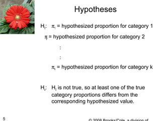
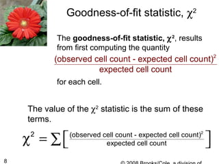
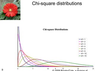
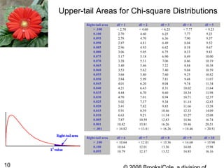
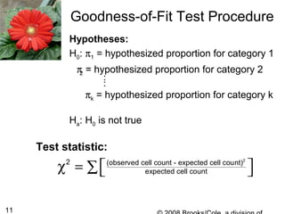
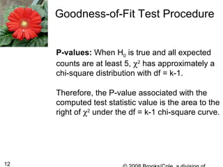
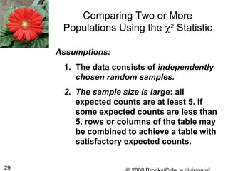
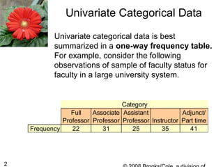
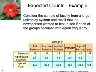
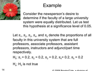
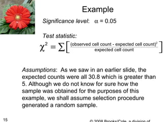
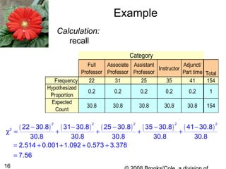
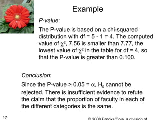
1. The document discusses categorical data analysis and goodness-of-fit tests. It introduces concepts such as univariate categorical data, expected counts, the chi-square test statistic, and assumptions of the chi-square test. 2. An example analyzes faculty status data from a university using a goodness-of-fit test to determine if the proportions are equal across categories. The test fails to reject the null hypothesis that the proportions are equal. 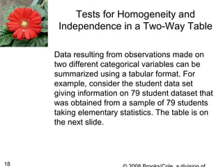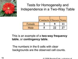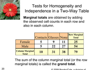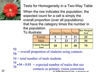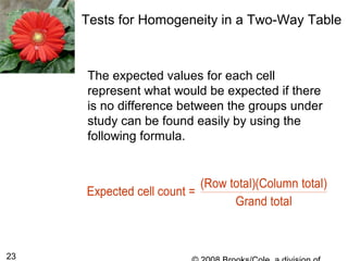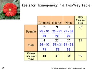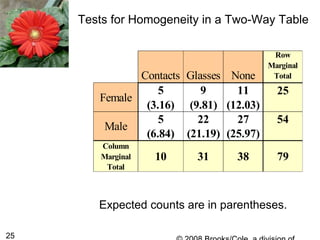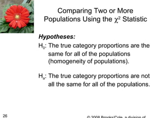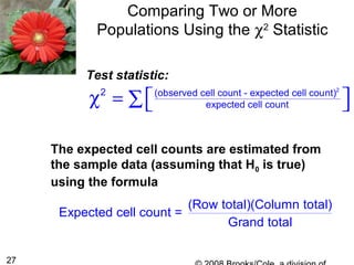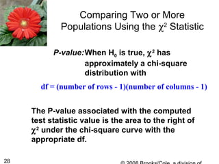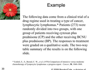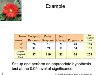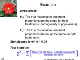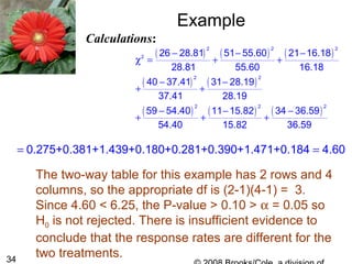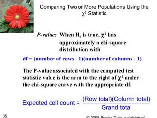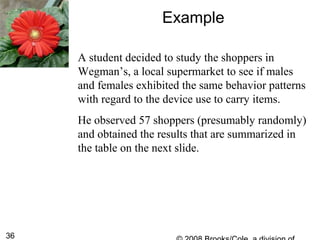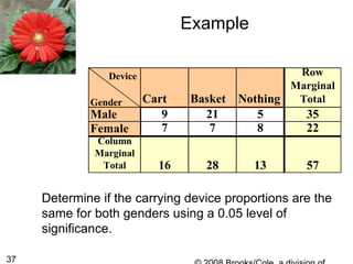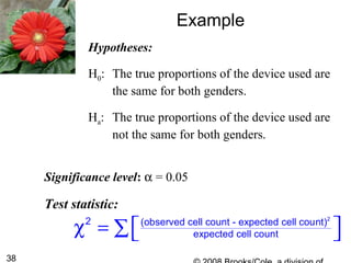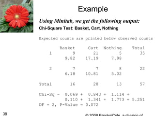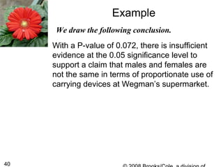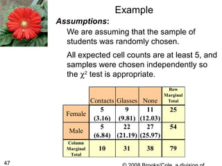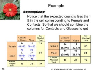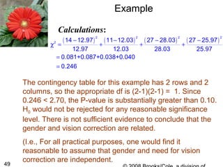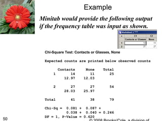3. Tests for homogeneity and independence in two-way tables are described. Examples calculate expected counts and perform chi-square tests to compare populations' category proportions.

1. 1
Chapter 12
The Analysis of Categorical Data
and
Goodness-of-Fit Tests

2. 2
Univariate Categorical Data
Univariate categorical data is best
summarized in a one-way frequency table.
For example, consider the following
observations of sample of faculty status for
faculty in a large university system.
Full
Professor
Associate
Professor
Assistant
Professor Instructor
Adjunct/
Part time
Frequency 22 31 25 35 41
Category

3. 3
Univariate Categorical Data
A local newsperson might be interested in
testing hypotheses about the proportion of
the population that fall in each of the
categories.
For example, the newsperson might want to
test to see if the five categories occur with
equal frequency throughout the whole
university system.
To deal with this type of question we need
to establish some notation.

4. 4
Notation
k = number of categories of a categorical variable
π1 = true proportion for category 1
π2 = true proportion for category 2
:
:
πk = true proportion for category k
(note: π1 + π2 + … + πk = 1)

5. 5
Hypotheses
H0: π1 = hypothesized proportion for category 1
π2 = hypothesized proportion for category 2
:
:
πk = hypothesized proportion for category k
Ha: H0 is not true, so at least one of the true
category proportions differs from the
corresponding hypothesized value.

6. 6
Expected Counts
For each category, the expected count for
that category is the product of the total
number of observations with the
hypothesized proportion for that category.

7. 7
Expected Counts - Example
Consider the sample of faculty from a large
university system and recall that the
newsperson wanted to test to see if each of
the groups occurred with equal frequency.
Full
Professor
Associate
Professor
Assistant
Professor
Instructor
Adjunct/
Part time Total
Frequency 22 31 25 35 41 154
Hypothesized
Proportion
0.2 0.2 0.2 0.2 0.2 1
Expected
Count
30.8 30.8 30.8 30.8 30.8 154
Category

8. 8
Goodness-of-fit statistic, χ2
The value of the χ2
statistic is the sum of these
terms.
The goodness-of-fit statistic, χ2
, results
from first computing the quantity
for each cell.
2
(observed cell count - expected cell count)
expected cell count
2
2 (observed cell count - expected cell count)
expected cell countχ =   ∑

9. 9
Chi-square distributions
Chi-square Distributions
0 5 10 15 20 25x
df = 1
df = 2
df = 3
df = 4
df = 5
df = 8
df = 10
df = 15

10. 10
Upper-tail Areas for Chi-square Distributions
Right-tail area df = 1 df = 2 df = 3 df = 4 df = 5
> .100 < 2.70 < 4.60 < 6.25 < 7.77 < 9.23
0.100 2.70 4.60 6.25 7.77 9.23
0.095 2.78 4.70 6.36 7.90 9.37
0.090 2.87 4.81 6.49 8.04 9.52
0.085 2.96 4.93 6.62 8.18 9.67
0.080 3.06 5.05 6.75 8.33 9.83
0.075 3.17 5.18 6.90 8.49 10.00
0.070 3.28 5.31 7.06 8.66 10.19
0.065 3.40 5.46 7.22 8.84 10.38
0.060 3.53 5.62 7.40 9.04 10.59
0.055 3.68 5.80 7.60 9.25 10.82
0.050 3.84 5.99 7.81 9.48 11.07
0.045 4.01 6.20 8.04 9.74 11.34
0.040 4.21 6.43 8.31 10.02 11.64
0.035 4.44 6.70 8.60 10.34 11.98
0.030 4.70 7.01 8.94 10.71 12.37
0.025 5.02 7.37 9.34 11.14 12.83
0.020 5.41 7.82 9.83 11.66 13.38
0.015 5.91 8.39 10.46 12.33 14.09
0.010 6.63 9.21 11.34 13.27 15.08
0.005 7.87 10.59 12.83 14.86 16.74
0.001 10.82 13.81 16.26 18.46 20.51
< .001 > 10.82 > 13.81 > 16.26 > 18.46 > 20.51
Right-tail area df = 6 df = 7 df = 8 df = 9 df = 10
> .100 < 10.64 < 12.01 < 13.36 < 14.68 < 15.98
0.100 10.64 12.01 13.36 14.68 15.98
0.095 10.79 12.17 13.52 14.85 16.16
0.090 10.94 12.33 13.69 15.03 16.35
0.085 11.11 12.50 13.87 15.22 16.54
0.080 11.28 12.69 14.06 15.42 16.75

11. 11
Goodness-of-Fit Test Procedure
Hypotheses:
H0: π1 = hypothesized proportion for category 1
π2 = hypothesized proportion for category 2
:
:
πk = hypothesized proportion for category k
Ha: H0 is not true
Test statistic:
2
2 (observed cell count - expected cell count)
expected cell countχ =   ∑

12. 12
Goodness-of-Fit Test Procedure
P-values: When H0 is true and all expected
counts are at least 5, χ2
has approximately a
chi-square distribution with df = k-1.
Therefore, the P-value associated with the
computed test statistic value is the area to the
right of χ2
under the df = k-1 chi-square curve.

13. 13
Goodness-of-Fit Test Procedure
Assumptions:
1. Observed cell counts are based on
a random sample.
2. The sample size is large. The
sample size is large enough for the
chi-squared test to be appropriate
as long as every expected count is
at least 5.

14. 14
Example
Consider the newsperson’s desire to
determine if the faculty of a large university
system were equally distributed. Let us test
this hypothesis at a significance level of 0.05.
Let π1, π2, π3, π4, and π5 denote the proportions of all
faculty in this university system that are full
professors, associate professors, assistant
professors, instructors and adjunct/part time
respectively.
H0: π1 = 0.2, π2 = 0.2, π3 = 0.2, π4= 0.2, π5 = 0.2
Ha: H0 is not true

15. 15
Example
Significance level: α = 0.05
Assumptions: As we saw in an earlier slide, the
expected counts were all 30.8 which is greater than
5. Although we do not know for sure how the
sample was obtained for the purposes of this
example, we shall assume selection procedure
generated a random sample.
Test statistic:
2
2 (observed cell count - expected cell count)
expected cell countχ =   ∑

16. 16
Example
Full
Professor
Associate
Professor
Assistant
Professor
Instructor
Adjunct/
Part time Total
Frequency 22 31 25 35 41 154
Hypothesized
Proportion
0.2 0.2 0.2 0.2 0.2 1
Expected
Count
30.8 30.8 30.8 30.8 30.8 154
Category
Calculation:
recall
( ) ( ) ( ) ( ) ( )
2 2 2 2 2
2 22 30.8 31 30.8 25 30.8 35 30.8 41 30.8
30.8 30.8 30.8 30.8 30.8
2.514 0.001 1.092 0.573 3.378
7.56
− − − − −
χ = + + + +
= + + + +
=

17. 17
Example
P-value:
The P-value is based on a chi-squared
distribution with df = 5 - 1 = 4. The computed
value of χ2
, 7.56 is smaller than 7.77, the
lowest value of χ2
in the table for df = 4, so
that the P-value is greater than 0.100.
Conclusion:
Since the P-value > 0.05 = α, H0 cannot be
rejected. There is insufficient evidence to refute
the claim that the proportion of faculty in each of
the different categories is the same.

18. 18
Tests for Homogeneity and
Independence in a Two-Way Table
Data resulting from observations made on
two different categorical variables can be
summarized using a tabular format. For
example, consider the student data set
giving information on 79 student dataset that
was obtained from a sample of 79 students
taking elementary statistics. The table is on
the next slide.

19. 19
Tests for Homogeneity and
Independence in a Two-Way Table
Contacts Glasses None
Female 5 9 11
Male 5 22 27
This is an example of a two-way frequency
table, or contingency table.
The numbers in the 6 cells with clear
backgrounds are the observed cell counts.

20. 20
Tests for Homogeneity and
Independence in a Two-Way Table
Contacts Glasses None
Row Marginal
Total
Female 5 9 11 25
Male 5 22 27 54
Column Marginal
Total
10 31 38 79
Marginal totals are obtained by adding
the observed cell counts in each row and
also in each column.
The sum of the column marginal total (or the row
marginal totals) is called the grand total.

21. 21
Tests for Homogeneity in a Two-Way Table
Typically, with a two-way table used to test
homogeneity, the rows indicate different
populations and the columns indicate
different categories or vice versa.
For a test of homogeneity, the central
question is whether the category proportions
are the same for all of the populations

22. 22
Tests for Homogeneity in a Two-Way Table
When the row indicates the population, the
expected count for a cell is simply the
overall proportion (over all populations)
that have the category times the number in
the population.
To illustrate: Contacts Glasses None
Row Marginal
Total
Female 5 9 11 25
Male 5 22 27 54
Column Marginal
Total
10 31 38 79
54 = total number of male students
= overall proportion of students using contacts
10
79
= expected number of males that use
contacts as primary vision correction
10
54 6.83
79
• =

23. 23
Tests for Homogeneity in a Two-Way Table
The expected values for each cell
represent what would be expected if there
is no difference between the groups under
study can be found easily by using the
following formula.
(Row total)(Column total)
Expected cell count =
Grand total

24. 24
Contacts Glasses None
Row
Marginal
Total
5 9 11
5 22 27
Column
Marginal
Total
10 31 38 79
Female
Male
25
54
×25 10
79
×25 31
79
×25 38
79
×54 10
79
×54 31
79
×54 38
79
Tests for Homogeneity in a Two-Way Table

25. 25
Contacts Glasses None
Row
Marginal
Total
5 9 11
(3.16) (9.81) (12.03)
5 22 27
(6.84) (21.19) (25.97)
Column
Marginal
Total
10 31 38 79
Female
25
Male
54
Tests for Homogeneity in a Two-Way Table
Expected counts are in parentheses.

26. 26
Comparing Two or More
Populations Using the χ2
Statistic
Hypotheses:
H0: The true category proportions are the
same for all of the populations
(homogeneity of populations).
Ha: The true category proportions are not
all the same for all of the populations.

27. 27
Comparing Two or More
Populations Using the χ2
Statistic
The expected cell counts are estimated from
the sample data (assuming that H0 is true)
using the formula
(Row total)(Column total)
Expected cell count =
Grand total
Test statistic:
2
2 (observed cell count - expected cell count)
expected cell countχ =   ∑

28. 28
Comparing Two or More
Populations Using the χ2
Statistic
P-value:When H0 is true, χ2
has
approximately a chi-square
distribution with
The P-value associated with the computed
test statistic value is the area to the right of
χ2
under the chi-square curve with the
appropriate df.
df = (number of rows - 1)(number of columns - 1)

29. 29
Comparing Two or More
Populations Using the χ2
Statistic
Assumptions:
1. The data consists of independently
chosen random samples.
2. The sample size is large: all
expected counts are at least 5. If
some expected counts are less than
5, rows or columns of the table may
be combined to achieve a table with
satisfactory expected counts.

30. 30
Example
The following data come from a clinical trial of a
drug regime used in treating a type of cancer,
lymphocytic lymphomas.* Patients (273) were
randomly divided into two groups, with one
group of patients receiving cytoxan plus
prednisone (CP) and the other receiving BCNU
plus prednisone (BP). The responses to treatment
were graded on a qualitative scale. The two-way
table summary of the results is on the following
slide.
* Ezdinli, E., S., Berard, C. W., et al. (1976) Comparison of intensive versus moderate
chemotherapy of lympocytic lymphomas: a progress report. Cancer, 38, 1060-1068.

31. 31
Example
Set up and perform an appropriate hypothesis
test at the 0.05 level of significance.
Complete
Response
Partial
Response
No
Change Progression
Row
Marginal
Total
26 51 21 40
31 59 11 34
Column
Marginal
Total
57 110 32 74 273
BP
CP
138
135

32. 32
Hypotheses:
H0: The true response to treatment
proportions are the same for both
treatments (homogeneity of populations).
Ha: The true response to treatment
proportions are not all the same for both
treatments.
Example
Significance level: α = 0.05
Test statistic:
2
2 (observed cell count - expected cell count)
expected cell countχ =   ∑

33. 33
Example
Assumptions:
All expected cell counts are at least 5, and
samples were chosen independently so the χ2
test is appropriate.

34. 34
Example
Calculations:
The two-way table for this example has 2 rows and 4
columns, so the appropriate df is (2-1)(4-1) = 3.
Since 4.60 < 6.25, the P-value > 0.10 > α = 0.05 so
H0 is not rejected. There is insufficient evidence to
conclude that the response rates are different for the
two treatments.
( ) ( ) ( )
( ) ( )
( ) ( ) ( )
− − −
χ = + +
− −
+ +
− − −
+ + +
2 2 2
2
2 2
2 2 2
26 28.81 51 55.60 21 16.18
28.81 55.60 16.18
40 37.41 31 28.19
37.41 28.19
59 54.40 11 15.82 34 36.59
54.40 15.82 36.59
= =0.275+0.381+1.439+0.180+0.281+0.390+1.471+0.184 4.60

35. 35
Comparing Two or More Populations Using the
χ2
Statistic
P-value: When H0 is true, χ2
has
approximately a chi-square
distribution with
df = (number of rows - 1)(number of columns - 1)
The P-value associated with the computed test
statistic value is the area to the right of χ2
under
the chi-square curve with the appropriate df.
(Row total)(Column total)
Expected cell count =
Grand total

36. 36
Example
A student decided to study the shoppers in
Wegman’s, a local supermarket to see if males
and females exhibited the same behavior patterns
with regard to the device use to carry items.
He observed 57 shoppers (presumably randomly)
and obtained the results that are summarized in
the table on the next slide.

37. 37
Example
Determine if the carrying device proportions are the
same for both genders using a 0.05 level of
significance.
Device
Gender Cart Basket Nothing
Row
Marginal
Total
Male 9 21 5 35
Female 7 7 8 22
Column
Marginal
Total 16 28 13 57

38. 38
Hypotheses:
H0: The true proportions of the device used are
the same for both genders.
Ha: The true proportions of the device used are
not the same for both genders.
Example
Significance level: α = 0.05
Test statistic:
2
2 (observed cell count - expected cell count)
expected cell countχ =   ∑

39. 39
Using Minitab, we get the following output:
Example
Chi-Square Test: Basket, Cart, Nothing
Expected counts are printed below observed counts
Basket Cart Nothing Total
1 9 21 5 35
9.82 17.19 7.98
2 7 7 8 22
6.18 10.81 5.02
Total 16 28 13 57
Chi-Sq = 0.069 + 0.843 + 1.114 +
0.110 + 1.341 + 1.773 = 5.251
DF = 2, P-Value = 0.072

40. 40
We draw the following conclusion.
Example
With a P-value of 0.072, there is insufficient
evidence at the 0.05 significance level to
support a claim that males and females are
not the same in terms of proportionate use of
carrying devices at Wegman’s supermarket.

41. 41
Hypotheses:
H0: The two variables are independent.
Ha: The two variables are not independent.
χ2
Test for Independence
The χ2
test statistic and procedures can also
be used to investigate the association
between tow categorical variable in a single
population.

42. 42
The expected cell counts are estimated from
the sample data (assuming that H0 is true)
using the formula
χ2
Test for Independence
Test statistic:
2
2 (observed cell count - expected cell count)
expected cell countχ =   ∑
(Row total)(Column total)
Expected cell count =
Grand total

43. 43
χ2
Test for Independence
The P-value associated with the computed
test statistic value is the area to the right of
χ2
under the chi-square curve with the
appropriate df.
(Row total)(Column total)
Expected cell count =
Grand total
P-value:When H0 is true, χ2
has
approximately a chi-square
distribution with
df = (number of rows - 1)(number of columns - 1)

44. 44
Assumptions:
1. The observed counts are from a
random sample.
2. The sample size is large: all
expected counts are at least 5. If
some expected counts are less
than 5, rows or columns of the
table may be combined to achieve
a table with satisfactory expected
counts.
χ2
Test for Independence

45. 45
Example
Consider the two categorical variables,
gender and principle form of vision
correction for the sample of students used
earlier in this presentation.
We shall now test to see if the gender and the
principle form of vision correction are independent.

46. 46
Example
Hypotheses:
H0: Gender and principle method of vision
correction are independent.
Ha: Gender and principle method of
vision correction are not independent.
Significance level: We have not chosen one,
so we shall look at the practical
significance level.
Test statistic:
2
2 (observed cell count - expected cell count)
expected cell countχ =   ∑

47. 47
Example
Assumptions:
We are assuming that the sample of
students was randomly chosen.
All expected cell counts are at least 5, and
samples were chosen independently so
the χ2
test is appropriate.
Contacts Glasses None
Row
Marginal
Total
5 9 11
(3.16) (9.81) (12.03)
5 22 27
(6.84) (21.19) (25.97)
Column
Marginal
Total
10 31 38 79
Female
25
Male
54

48. 48
Example
Assumptions:
Notice that the expected count is less than
5 in the cell corresponding to Female and
Contacts. So that we should combine the
columns for Contacts and Glasses to get
Contacts
or Glasses None
Row
Marginal
Total
14 11
(12.97) (12.03)
27 27
(28.03) (25.97)
Column
Marginal
Total
41 38 79
Female 25
Male 54
Contacts
or Glasses None
Row
Marginal
Total
14 11
27 27
Column
Marginal
Total
41 38 79
Female
25
Male
54
×41 25
79
×38 25
79
×41 54
79
×38 54
79

49. 49
Example
The contingency table for this example has 2 rows and 2
columns, so the appropriate df is (2-1)(2-1) = 1. Since
0.246 < 2.70, the P-value is substantially greater than 0.10.
H0 would not be rejected for any reasonable significance
level. There is not sufficient evidence to conclude that the
gender and vision correction are related.
(I.e., For all practical purposes, one would find it
reasonable to assume that gender and need for vision
correction are independent.
Calculations:
( ) ( ) ( ) ( )
2 2 2 2
2 14 12.97 11 12.03 27 28.03 27 25.97
12.97 12.03 28.03 25.97
0.081+0.087+0.038+0.040
0.246
− − − −
χ = + + +
=
=

50. 50
Example
Minitab would provide the following output
if the frequency table was input as shown.
Chi-Square Test: Contacts or Glasses, None
Expected counts are printed below observed counts
Contacts None Total
1 14 11 25
12.97 12.03
2 27 27 54
28.03 25.97
Total 41 38 79
Chi-Sq = 0.081 + 0.087 +
0.038 + 0.040 = 0.246
DF = 1, P-Value = 0.620