Download as PDF, PPTX

![The Binomial Distribution: Example
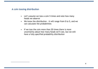
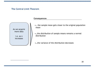
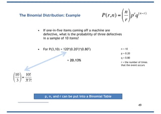
• If one-in-five items coming off a machine are
defective, what is the probability of three or more
defectives in a sample of 10 items?
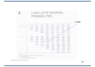
• For P(0,10) = 1*(0.200)*(0.8010) = 0.1073
• For P(1,10) = 10*(0.201)*(0.809)
• For P(2,10) = 45*(0.202)*(0.808)
• P(>=3) = 1 – [P(2)+P(1)+P(0)]
= 1 – 0.678
= 32.2%
n = 10
p = 0.20
q = 0.80
r = the number of times
that the event occurs
p, n, and r can be put into a Binomial Table
34
€
P(r,n) =
n
r
"
#
$
%
&
'pr
q(n−r)](https://image.slidesharecdn.com/probabilitydistributionss-181220094651/85/Probability-Distributions-34-320.jpg)

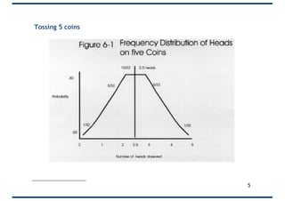
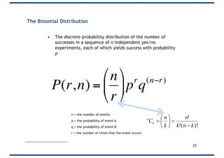
![The Binomial Distribution: Example
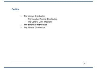
• If one-in-five items coming off a machine are
defective, what is the probability of three or more
defectives in a sample of 10 items?
• For P(0,10) = 1*(0.200)*(0.8010) = 0.1073
• For P(1,10) = 10*(0.201)*(0.809)
• For P(2,10) = 45*(0.202)*(0.808)
• P(>=3) = 1 – [P(2)+P(1)+P(0)]
= 1 – 0.678
= 32.2%
n = 10
p = 0.20
q = 0.80
r = the number of times
that the event occurs
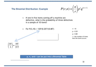
p, n, and r can be put into a Binomial Table
50
€
P(r,n) =
n
r
"
#
$
%
&
'pr
q(n−r)](https://image.slidesharecdn.com/probabilitydistributionss-181220094651/85/Probability-Distributions-50-320.jpg)
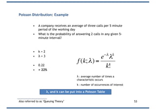


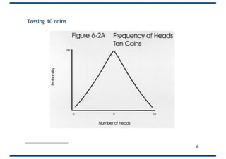
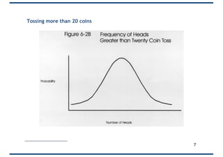
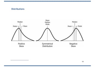
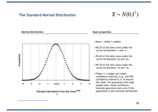
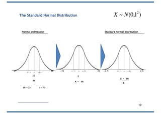
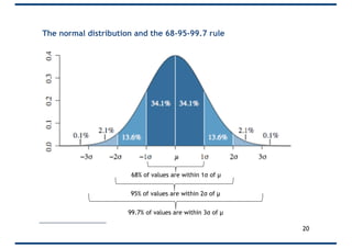
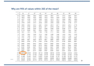
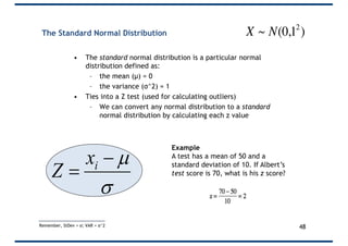
The document covers probability distributions, focusing on normal, binomial, and Poisson distributions, along with the central limit theorem. It explains how to read and apply these distributions in practical scenarios, including examples involving coin tossing and customer arrivals. Students are expected to develop an understanding of these concepts and their applications in statistics.


![[DSC Europe 25] Bojan Djuricic - Predictive Design Process.pdf](https://cdn.slidesharecdn.com/ss_thumbnails/5awdrbedqdek3gqu2ezy-4-the-predictive-design-bojan-djuricic-260120105856-6c399e9b-thumbnail.jpg?width=640&height=640&fit=bounds)
![[DSC Europe 25] Slobodan Dolinic - Smart and Intelligent Green Region.pptx](https://cdn.slidesharecdn.com/ss_thumbnails/0bribinjsp6ghwtvsvor-2-sigre-slobodan-dolinic-260115093812-c9c10e90-thumbnail.jpg?width=640&height=640&fit=bounds)


![[DSC Europe 25] Ivan Lukovic & Marija Djukic - From Data to Value: Why Maturi...](https://cdn.slidesharecdn.com/ss_thumbnails/ahrfps8xr6knowwhacxh-1-ivan-marija-dsc-2025-ld-v1-presentation-260115093812-be21adfc-thumbnail.jpg?width=640&height=640&fit=bounds)


![[DSC Europe 25] Andrzej Kowalczyk - AI - how to start small and grow in the f...](https://cdn.slidesharecdn.com/ss_thumbnails/oy1zmo94qv6vpcqjvno2-andrzej-kowalczyk-ai-how-to-start-small-and-grow-in-the-future-1-260119121559-cf093b23-thumbnail.jpg?width=640&height=640&fit=bounds)
![[DSC Europe 25] Elena Menshikova - AI-Powered Operational Excellence: Revolut...](https://cdn.slidesharecdn.com/ss_thumbnails/es6nholbqy3zaao2c2yd-2-elena-menshikova-data-ai-in-decision-making-260115093812-4fba8b38-thumbnail.jpg?width=640&height=640&fit=bounds)