Downloaded 70 times


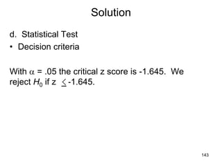


![Solution
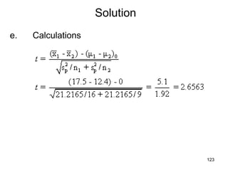
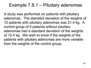
e. Calculations
s2 = .4*12 = 4.8
c2= [11(4.8)]/4=13.2
169](https://image.slidesharecdn.com/hypothesistesting-191026160454/85/Hypothesis-testing-169-320.jpg)


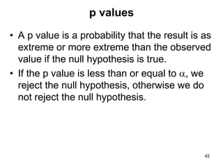
The document discusses hypothesis testing, a statistical procedure used to draw conclusions about populations based on sample data, emphasizing its importance in fields like medicine and biology. It defines key concepts such as null and alternative hypotheses, significance levels, and types of errors, and outlines a structured procedure for conducting hypothesis tests including formulation of hypotheses, selection of test statistics, and interpretation of results. Additionally, it covers specific examples of hypothesis testing for population means, differences between two means, and assumptions necessary for valid conclusions.