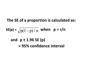
Standard Error & Confidence
Intervals
The basic problems to which Statistics
are applied in practice arise when trying
to deduce something about a population
from the evidence provided by a sample
of observations taken from that
population.
Our measurements
may give rise to a
certain amount of
uncertainty which
is measured as
probability.
The population
parameters do not change
and remain constant
whereas the sample
estimates can change and
take any random value.
Population Sample
parameters estimates
Mean μ
Standard
deviation σ SD
Proportion π p
Population
correlation
coefficient ρ r
x
The mathematical nature of
probability is defined as the
proportion of times that a
certain outcome would occur
if we repeated the experiment
or observation a large number
of times under similar
conditions.
A probability is somewhat
similar to a proportion: an
outcome is 0.29 means a
probability of an event to occur
is 29%. Probabilities are
expressed as percentages.
Because probabilities are
defined to be proportions, a
probability should be between
0 and 1.
The sum of all possible
events is 1. Any breakdown
of the total probability of
each of the events is called a
probability distribution.
10
THE NORMAL DISTRIBUTION
• Many variables have a normal distribution.
This is a bell shaped curve with most of the
values clustered near the mean and a few
values out near the tails.
11
THE NORMAL DISTRIBUTION
12
13
• The normal distribution is symmetrical around the
mean. The mean, the median and the mode of a
normal distribution have the same value.
THE RELATION OF THE SAMPLE TO THE
WHOLE POPULATION
• When you undertake a study, it is usually
necessary to draw a sample from the study
population.
• You will then describe the population on the
basis of the information collected from the
sample.
• In other words, you will try to generalize the
findings from the sample to the larger
population. Obviously, this can be done if
the sample is selected in such a way that it
can be considered representative of the
whole population.
• Any value of a variable obtained from the
sample (e.g. a mean) can then be considered
as an estimate of the corresponding
population value.
• For example, if 158 cm is the calculated mean height of a
sample of 120 women you hope it is a good
approximation of the mean height of the population of
women as a whole.
• However, the sample mean is not likely to be identical to
the population mean.
• If you draw another sample of 120 mothers, you might
find a mean of 157 cm, which is not identical to the first
sample mean. It probably also differs from the true mean
height of the total population from which the sample
was drawn.
• This phenomenon is called SAMPLING VARIATION.
• HOW TO DETERMINE THE EXTENT TO
WHICH THE SAMPLE REPRESENTS THE
POPULATION AS A WHOLE.
• To find out to what extent a particular
sample value deviates from the population
value, a range or an interval around the
sample value can be worked out which will
most probably contain the population
value.
• This range or interval is called the
CONFIDENCE INTERVAL.
• The calculation of a confidence interval
takes into account the STANDARD ERROR.
• The standard error gives an estimate of
the degree to which the sample mean
varies from the population means. It is
computed on the basis of the standard
deviation.
• The standard error for the mean is
calculated by dividing the standard
deviation by the square root of the sample
size:
• standard deviation/ √Sample size
or SD / n
95% CONFIDENCE INTERVAL
• When describing variables statistically you
usually present the calculated sample mean
1.96 times the SE( ).
• This is then called the 95% CONFIDENCE
INTERVAL. It means that there is 95%
probability that the population mean lies
within this interval.
x
• Note that the larger the sample size, the
smaller the standard error and the narrower
the confidence interval will be. Thus the
advantage of having a large sample size is
that the sample mean will be a better
estimate of the population mean.
Eg., Consider a population with five
digits: 2, 3, 4, 5, 6
= 2+3+4+5+6/5=20/5=4.0
= (2-4)2+(3-4)2+(4-4)2+(5-4)2
+(6-4)2 /5 = = 1.414


2
If all possible samples of size (n=2)
are drawn from this population:
52 = 25 samples:
2,2 2,3 2,4 2,5 2,6
3,2 3,3 3,4 3,5 3,6
4,2 4,3 4,4 4,5 4,6
5,2 5,3 5,4 5,5 5,6
6,2 6,3 6,4 6,5 6,6
If means are calculated for each
sample:
2.0 2.5 3.0 3.5 4.0
2.5 3.0 3.5 4.0 4.5
3.0 3.5 4.0 4.5 5.0
3.5 4.0 4.5 5.0 5.5
4.0 4.5 5.0 5.5 6.0
The Mean of these 25 means = 4.0
x
The Mean (of these 25 means =
4.0 which is equal to the population
mean ( = 4.0) . This shows that the
Mean of the means is a good
estimator of population mean .
But,

x

x
The Standard Deviation of these 25
means = 1.0 instead of
= 1.414
This value is actually equal to
another property = / i.e.,
1.414/ =1.0 This is called the
Standard error (SE) of the sampling
distribution of the means.
x


 n
2
x
2 6
4
0
5
The SE of a proportion is calculated as:
SE(p) = when p = r/n
and p ± 1.96 SE (p)
= 95% confidence interval
n
/
p)
p(1

Standard Error & Confidence Intervals.pptx

  • 1.
    Standard Error &Confidence Intervals
  • 2.
    The basic problemsto which Statistics are applied in practice arise when trying to deduce something about a population from the evidence provided by a sample of observations taken from that population.
  • 3.
    Our measurements may giverise to a certain amount of uncertainty which is measured as probability.
  • 4.
    The population parameters donot change and remain constant whereas the sample estimates can change and take any random value.
  • 5.
    Population Sample parameters estimates Meanμ Standard deviation σ SD Proportion π p Population correlation coefficient ρ r x
  • 6.
    The mathematical natureof probability is defined as the proportion of times that a certain outcome would occur if we repeated the experiment or observation a large number of times under similar conditions.
  • 7.
    A probability issomewhat similar to a proportion: an outcome is 0.29 means a probability of an event to occur is 29%. Probabilities are expressed as percentages.
  • 8.
    Because probabilities are definedto be proportions, a probability should be between 0 and 1.
  • 9.
    The sum ofall possible events is 1. Any breakdown of the total probability of each of the events is called a probability distribution.
  • 10.
    10 THE NORMAL DISTRIBUTION •Many variables have a normal distribution. This is a bell shaped curve with most of the values clustered near the mean and a few values out near the tails.
  • 11.
  • 12.
  • 13.
    13 • The normaldistribution is symmetrical around the mean. The mean, the median and the mode of a normal distribution have the same value.
  • 14.
    THE RELATION OFTHE SAMPLE TO THE WHOLE POPULATION • When you undertake a study, it is usually necessary to draw a sample from the study population. • You will then describe the population on the basis of the information collected from the sample.
  • 15.
    • In otherwords, you will try to generalize the findings from the sample to the larger population. Obviously, this can be done if the sample is selected in such a way that it can be considered representative of the whole population. • Any value of a variable obtained from the sample (e.g. a mean) can then be considered as an estimate of the corresponding population value.
  • 16.
    • For example,if 158 cm is the calculated mean height of a sample of 120 women you hope it is a good approximation of the mean height of the population of women as a whole. • However, the sample mean is not likely to be identical to the population mean. • If you draw another sample of 120 mothers, you might find a mean of 157 cm, which is not identical to the first sample mean. It probably also differs from the true mean height of the total population from which the sample was drawn. • This phenomenon is called SAMPLING VARIATION.
  • 17.
    • HOW TODETERMINE THE EXTENT TO WHICH THE SAMPLE REPRESENTS THE POPULATION AS A WHOLE.
  • 18.
    • To findout to what extent a particular sample value deviates from the population value, a range or an interval around the sample value can be worked out which will most probably contain the population value. • This range or interval is called the CONFIDENCE INTERVAL.
  • 19.
    • The calculationof a confidence interval takes into account the STANDARD ERROR. • The standard error gives an estimate of the degree to which the sample mean varies from the population means. It is computed on the basis of the standard deviation.
  • 20.
    • The standarderror for the mean is calculated by dividing the standard deviation by the square root of the sample size: • standard deviation/ √Sample size or SD / n
  • 21.
    95% CONFIDENCE INTERVAL •When describing variables statistically you usually present the calculated sample mean 1.96 times the SE( ). • This is then called the 95% CONFIDENCE INTERVAL. It means that there is 95% probability that the population mean lies within this interval. x
  • 22.
    • Note thatthe larger the sample size, the smaller the standard error and the narrower the confidence interval will be. Thus the advantage of having a large sample size is that the sample mean will be a better estimate of the population mean.
  • 23.
    Eg., Consider apopulation with five digits: 2, 3, 4, 5, 6 = 2+3+4+5+6/5=20/5=4.0 = (2-4)2+(3-4)2+(4-4)2+(5-4)2 +(6-4)2 /5 = = 1.414   2
  • 24.
    If all possiblesamples of size (n=2) are drawn from this population: 52 = 25 samples: 2,2 2,3 2,4 2,5 2,6 3,2 3,3 3,4 3,5 3,6 4,2 4,3 4,4 4,5 4,6 5,2 5,3 5,4 5,5 5,6 6,2 6,3 6,4 6,5 6,6
  • 25.
    If means arecalculated for each sample: 2.0 2.5 3.0 3.5 4.0 2.5 3.0 3.5 4.0 4.5 3.0 3.5 4.0 4.5 5.0 3.5 4.0 4.5 5.0 5.5 4.0 4.5 5.0 5.5 6.0 The Mean of these 25 means = 4.0 x
  • 26.
    The Mean (ofthese 25 means = 4.0 which is equal to the population mean ( = 4.0) . This shows that the Mean of the means is a good estimator of population mean . But,  x  x
  • 27.
    The Standard Deviationof these 25 means = 1.0 instead of = 1.414 This value is actually equal to another property = / i.e., 1.414/ =1.0 This is called the Standard error (SE) of the sampling distribution of the means. x    n 2 x
  • 28.
  • 29.
    The SE ofa proportion is calculated as: SE(p) = when p = r/n and p ± 1.96 SE (p) = 95% confidence interval n / p) p(1