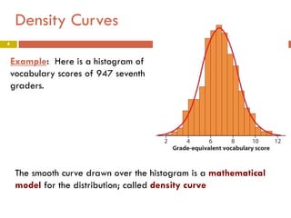
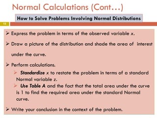
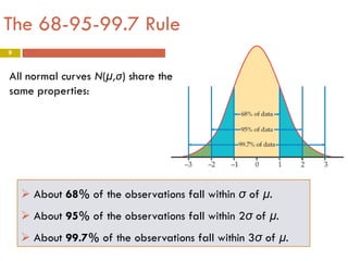
1) The document discusses density curves and normal distributions, which are important mathematical models for describing the overall pattern of data. A density curve describes the distribution of a large number of observations. 2) It specifically covers the normal distribution and some of its key properties, including that about 68%, 95%, and 99.7% of observations fall within 1, 2, and 3 standard deviations of the mean, respectively. 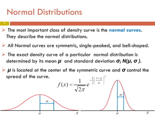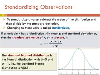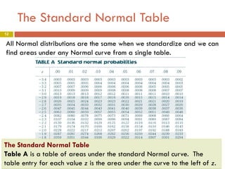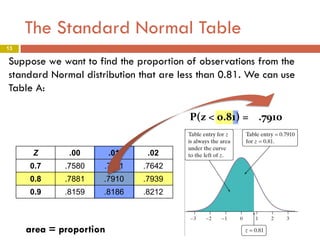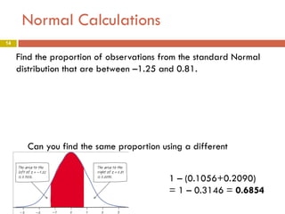3) The document shows how to work with normal distributions using techniques like standardizing data, finding areas under the normal curve using the standard normal table, and assessing normality with a normal quantile plot.

1. 1
INTRODUCTION TO
STATISTICS & PROBABILITY
Chapter 1:
Looking at Data—Distributions (Part 3)
1.3 Density Curves and Normal Distributions
Dr. Nahid Sultana

2. 2
1.3 Density Curves and Normal
Distributions
Objectives
 Density curves
 Measuring center and spread for density curves
 Normal distributions
 The 68-95-99.7 rule
 Standardizing observations
 Using the standard Normal Table
 Inverse Normal calculations
 Normal quantile plots

3. Exploring Quantitative Data
3
Use graphical and numerical tools for describing distributions:
1. Always plot your data: make a graph (Histogram, stemplot);
2. Look for the overall pattern (shape, center, and spread) and
for striking deviations such as outliers;
3. Calculate a numerical summary to briefly describe center
and spread.
4. Sometimes the overall pattern of a large number of
observations is so regular that we can describe it by a
smooth curve.

4. Density Curves
4
Example: Here is a histogram of
vocabulary scores of 947 seventh
graders.
The smooth curve drawn over the histogram is a mathematical
model for the distribution; called density curve

5. Density Curves (Cont…)
5
A density curve is a curve that:
 is always on or above the horizontal axis
 has an area of exactly 1 underneath it
 A density curve describes the overall pattern of a distribution.
 The area under the curve and above any range of values on the
horizontal axis is the proportion of all observations that fall in that
range. In short,
area = proportion

6. Median and mean of a density curve
6
 The mean of a density curve is the balance point, at which the
curve would balance if it were made of solid material.
 The median of a density curve is the equal-areas point―the
point that divides the area under the curve in half.
 The mean and the median are the same for a symmetric density curve.
They both lie at the center of the curve.
 The mean of a skewed curve is pulled away from the median in the
direction of the long tail.

7. Normal Distributions
7
 The most important class of density curve is the normal curves.
They describe the normal distributions.
 All Normal curves are symmetric, single-peaked, and bell-shaped.
 The exact density curve of a particular normal distribution is
determined by its mean µ and standard deviation σ; N(µ, σ ).
 µ is located at the center of the symmetric curve and σ control the
spread of the curve.

8. A family of density curves
8

9. The 68-95-99.7 Rule
9
All normal curves N(µ,σ) share the
same properties:
 About 68% of the observations fall within σ of µ.
 About 95% of the observations fall within 2σ of µ.
 About 99.7% of the observations fall within 3σ of µ.

10. The 68-95-99.7 Rule (Cont…)
10
Example: In a recent year 76,531 tenth-grade Indiana students took
the English/language arts exam. The mean score was 572 and the
standard deviation was 51. Assuming that these scores are
approximately Normally distributed, N(572, 51).
Q. Use the 68–95–99.7 rule to give a range of scores that
includes 95% of these students.
Solution: 572 ± 2(51) i.e. 470 to 674.
Q. Use the 68–95–99.7 rule to give a range of scores that
includes 99.7% of these students.
Solution: 572 ± 3(51) i.e. 419 to 725

11. Standardizing Observations
11
 To standardize a value, subtract the mean of the distribution and
then divide by the standard deviation.
 Changing to these units is called standardizing.
If a variable x has a distribution with mean µ and standard deviation σ,
then the standardized value of x, or its z-score, is
x- μ
z =
σ
The standard Normal distribution is
the Normal distribution with µ=0 and
σ =1. i.e., the standard Normal
distribution is N(0,1).

12. The Standard Normal Table
12
All Normal distributions are the same when we standardize and we can
find areas under any Normal curve from a single table.
The Standard Normal Table
Table A is a table of areas under the standard Normal curve. The
table entry for each value z is the area under the curve to the left of z.

13. The Standard Normal Table
13
Suppose we want to find the proportion of observations from the
standard Normal distribution that are less than 0.81. We can use
Table A:
P(z < 0.81) = .7910
Z
.00
.01
.02
0.7
.7580
.7611
.7642
0.8
.7881
.7910
.7939
0.9
.8159
.8186
.8212
area = proportion
13

14. Normal Calculations
14
Find the proportion of observations from the standard Normal
distribution that are between –1.25 and 0.81.
Can you find the same proportion using a different
approach?
1 – (0.1056+0.2090)
= 1 – 0.3146 = 0.6854
14

15. Normal Calculations (Cont…)
How to Solve Problems Involving Normal Distributions
15
 Express the problem in terms of the observed variable x.
 Draw a picture of the distribution and shade the area of interest
under the curve.
 Perform calculations.
 Standardize x to restate the problem in terms of a standard
Normal variable z.
 Use Table A and the fact that the total area under the curve
is 1 to find the required area under the standard Normal
curve.
 Write your conclusion in the context of the problem.

16. Normal Calculations (Cont…)
16
According to the Health and Nutrition Examination Study of 1976–
1980, the heights (in inches) of adult men aged 18–24 are N(70, 2.8).
Q. How tall must a man be in the lower 10% for men aged 18–24?
N(70, 2.8)
.10
?
70

17. Normal Calculations (Cont…)
17
Q. How tall must a man be in the lower
10% for men aged 18–24?
N(70, 2.8)
.10
Solution:
 Look up the closest
probability (closest to 0.10) in
the table.
?
70
17
.07
.08
.09
−1.3
.0853
.0838
.0823
-1.2
.1020
.1003
.0985
−1.1
 Find the corresponding
standardized score.
z
.1210
.1190
.1170
Z = –1.28

18. Normal Calculations (Cont…)
18
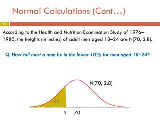
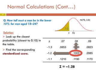
Q. How tall must a man be in the lower
10% for men aged 18–24?
N(70, 2.8)
.10
Solution: Cont…
? 70
We need to “unstandardize” the z-score to find the observed value x:
z=
x−µ
σ
x = µ + zσ
x = 70 + z (2.8)
= 70 + [(-1.28 ) × (2.8)]
= 70 + (−3.58) = 66.42
A man would have to be approximately 66.42 inches tall or less to
place in the lower 10% of all men in the population.

19. Normal Quantile Plots
19
One way to assess if a distribution is indeed approximately normal
is to plot the data on a normal quantile plot.
 If the distribution is indeed normal the plot will show a
straight line, indicating a good match between the data and a
normal distribution.
 Systematic deviations from a straight line indicate a nonnormal distribution. Outliers appear as points that are far
away from the overall pattern of the plot.

20. Normal Quantile Plots (Cont…)
20
Good fit to a straight line:
the distribution of rainwater
pH values is close to normal.
Curved pattern: the data are not
normally distributed.
Normal quantile plots are complex to do by hand, but they are
standard features in most statistical software.