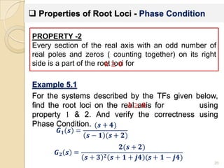
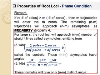
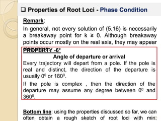
The document discusses root locus analysis and controller design techniques. 1) Root locus analysis involves plotting the trajectories of a system's closed-loop poles as a parameter (such as a controller gain) is varied. Properties of root loci like pole departure angles and asymptotes are examined. 2) Design specifications like overshoot and settling time can be translated to desired pole regions. A simple proportional controller can place poles near this region. 3) Additional controller types like integral and derivative are introduced to modify the root locus for improved steady-state response or damping. Combining controller types benefits stability.

1. Chapter 5: Root Locus Analysis
Outline
 Motivational Example
 desired pole region
 Simple controller design using desired pole
region
 Construction of Root Loci
 Magnitude condition
• Stability range from Root Loci
 phase condition
• properties of Root Loci
 Effects of addition of pole(s) and zero(s)
 Classical Dynamic Compensation
1

2.  Motivational Example
Consider a plant with TF
(5.1)
• The problem is to design an overall system to meet
the following specifications:
position error = 0
overshoot ≤ 5%
Settling time ≤ 8 seconds
Rise time as small as possible
• Before carrying out the design, we must first choose
a configuration and a compensator ( controller) with
one open parameter. The simplest possible FB
configuration & compensator are shown in Figure 5.1
2
1
2
3
4

3.  Motivational Example
5.1 Unity-feedback control system
• The overall TF ( for system in Fig 5.1) is
(5.2)
Note:
• is stable if and only if k>0
• Because , the system has zero position
error 3
+ K
-
Ctrl Plant
u yr e

4.  Motivational Example
Thus, the design reduces to the search for a positive
k to meet requirements (2) through (4)
Remark:
Design specifications are given in the time domain ,
whereas the design is carried out using TF’s , or in
the s-plane. Hence, a mapping relating transient
performance specifications and desired pole region
must be done!
Consider a control system with a TF
(5.3)
The overshoot is
4

5.  Desired pole region
• From Fig 5.2(b), the range of for a given
overshoot can be obtained.
5
5. 2 Damping ratio &
Overshoot
(a) (b)

6.  Desired pole region
• ( as defined in Fig 5.2(b))
• is a decreasing function of in
i.e., if , then
Example on translating overshoot specif. into a pole
region in the s-plane
• Overshoot ≤ 10%  
• Overshoot ≤ 5%  
6
Figure 5.3 Overshoot & pole
region

7.  Desired pole region
Translating settling time into a pole region in the s-
plane
7
Figure 5.4 Desired pole
region

8.  Desired pole region
Remarks:
• The translation of the rise time into a pole region can
not be done quantitatively as in the case of overshoot
and settling time.
• Generally, the farther away the closest pole from the
origin of the s-plane, the smaller the rise time.
8
Summary
Overshoot Sector with & is determined from Fig 5.2b
Settling
Time
Rise Time

9.  Simple controller design using desired pole region
Consider the design problem in Figure 5.1
9
Figure 5.5 Poles of
Gcl(s)
-2
2
1
-1
-2-3 -1 1
Re(s
)
Im(s)
K=0
K=.36K=.75
K=5
K=1
K=2

10.  Simple controller design using desired pole region
Consider the design problem in Figure 5.1…..
Q. How to choose k from 0.75, 1 and 2, so that the
rise time will be the smallest?
• the poles corresponding to k=0.75 are -0.5 & -1.5;
therefore, the distance of the closer pole from the
origin is 0.5
10
Gain Poles Comments
K=0.36 -0.2, -1.8 Meet (2) but not (3)
K=0.75 -0.5, -1.5 Meet both (2) & (3)*
K=1 -1,-1 Meet both (2) & (3)*
K=2 -1 j1 Meet both (2) & (3)*
K=5 -1 2j Meet (3) but not (2)

11.  Simple controller design using desired pole region
• the poles corresponding to k=1 are -1 and -1. Their
distance from the origin is 1 and is larger than 0.5.
• the poles corresponding to k=2 are -1± j1. their distance
from the origin is , which is the largest among
k=0.75, 1 and 2.
• Therefore, the system with k=2 has the smallest rise time
or, equivalently, responds faster.
Remark
If some of the specifications are more stringent, then no k
may exist. For example , if Ts< 2 sec, then all poles of
Gcl(s) must lie on the left-hand side of the vertical line
passing through -4/2=-2. From Figure 5.5 no poles meet
the requirement. In this case, we must choose a different
configuration and/or a more complicated compensator and
redesign. 11
Verify via Matlab Simulation!

12.  Simple controller design using desired pole region
A more systematic design method consists two major
components ;
(1) Translation of the transient performance into a
desired pole region. We then try to place the poles
of the overall system inside the region by
choosing a parameter.
(2) In order to facilitate the choice of the parameter,
the poles of the overall system as a function of the
parameter will be plotted graphically. Such plot is
called ROOT-LOCUS.
Reading assignment
Effects of introducing a zero/pole on the quadratic TF
with constant numerator(the details).
12

13.  Construction of Root-Locus
Consider the unity-feedback control system shown in
Fig 5.6, where G(s) is a proper rational function* and
k is a real constant.
Let
Then the overall TF is
13
Figure 5.6 Unity feedback
system
+ K G(s)
-
Ctrl Plant
u yr e

14.  Construction of Root-Locus
The poles of Gcl(s) are the zeros of the rational
function
(5.4) or the solution of the
eqn.
(5.5)
Definition 5.1
To simplify discussion, let assume
(5.6) ; q- real constant
Re-writing (5.5) as
14
The roots of D(s)+kN(s) or the poles of Gcl(s) as a
function of a real k are called the root loic.

15.  Construction of Root-Locus
Then the roots of D(s)+kN(s) are those s,
real/complex which satisfy (5.7) for some real k.
From Figure 5.7, we have
15
Figure 5.7 Vector in s-
plane

16.  Construction of Root-Locus
Substituting the above relations into (5.7) gives
(5.8)
Eqn.(5.8) consists of two parts; the magnitude
condition
(5.9)
And the phase condition
(5.10) 16

17.  Construction of Root-Locus
Note
• equals 0 if , if
• can be positive ( if measured
counterclockwise)
Phase Condition
Because k is real , we have
Note two angles will be considered the same if they
differ by ±2π radians ( or 3600) or their multiples.
Hence, (5.10) becomes
(5.11) Total phase:=
= 17

18.  Construction of Root-Locus
Conclusion
If s1 satisfy (5.11), then there exists a real k1 such that
D(s1)+k1N(s1)=0. This k1 can be computed from (5.9)
BIG QUESTION: How to search for s1?
ANSWER: Using the properties to be discussed
shortly, we can obtain a rough sketch of root loci
without any measurement.
Properties of Root Loic - Phase condition
Consider a TF with real coefficients expressed as
(5.12)
with
18

19.  Properties of Root Loci - Phase Condition
To simplify discussion, assume and in
(5.13)
Proof:
The polynomial in (5.13) has degree n. Thus for each
real k, there are n-roots. Because the roots of a
polynomial are continuous function of its coefficients,
the n-roots form n continuous trajectories as k varies
from 0 to .
19
PROPERTY -1
The root loci consists of n-continuous trajectories as k
varies continuously from 0 to . The trajectories are
symmetric w.r.t the real axis.

20.  Properties of Root Loci - Phase Condition
Example 5.1
For the systems described by the TFs given below,
find the root loci on the real axis for using
property 1 & 2. And verify the correctness using
Phase Condition.
20
PROPERTY -2
Every section of the real axis with an odd number of
real poles and zeros ( counting together) on its right
side is a part of the root loci for

21.  Properties of Root Loci - Phase Condition
Example 5.1…
21
Figure 5.8 Root Loci on real-
axis
S2=
0
2.
5
s1
-4 -2
1
Re(s
)
Im(s)
Asymptot
e
(a
)
600
-
600
-2-3 21
3.
5
Asymptot
e
Asymptot
e
Re(s
)
Im(s)
(b)

22.  Properties of Root Loci - Phase Condition
Example 5.1…
Remark:
The net phase due to the pair to any point on the real
axis equals 0 or 2π as shown in Figure 5.8(b).
Therefore, in applying property 2, complex-conjugate
poles and zeros can be disregarded.
Proof:
The roots of are the same as the
roots of .
22
PROPERTY -3
The n-trajectories migrate from the poles of G(s) to the
zeros of G(s) as k increases from 0 to .

23.  Properties of Root Loci - Phase Condition
Remark:
If n( # of poles) > m ( # of zeros) , then m trajectories
will enter the m zeros. The remaining (n-m)
trajectories will approach (n-m) asymptotes, as
discussed in property 4.
23
PROPERTY -4
For large s, the root loci will approach (n-m) number of
straight lines called asymptotes, emitting from
(5.14a)
called the centroid. These (n-m) asymptotes have
angles
(5.14b)
These formulas will give only (n-m) distinct angle.

24.  Properties of Root Loci - Phase Condition
Property 4 continued…
24
n-m Angles of
asymptotes
1 1800
2 ±900
3 ±600, 1800
4 ±450, ±1350
5 ±360, ±1080,1800
PROPERTY -5
Breakaway points- solution of
A breakaway point is where two roots collide and break
away; therefore, there are at least two roots at every
breakaway point.

25.  Properties of Root Loci - Phase Condition
Property 5 continued…
Proof:
Let s0 be a breakaway point of D(s)+kN(s). Then it is
a repeated root of D(s)+kN(s). Consequently, we
have
(5.15a) and
(5.15b)
Solving for k from (5.15b) and substituting into (5.15a)
gives

(5.16) 25

26.  Properties of Root Loci - Phase Condition
Remark:
In general, not every solution of (5.16) is necessarily
a breakaway point for k ≥ 0. Although breakaway
points occur mostly on the real axis, they may appear
elsewhere.
Bottom line: using the properties discussed so far, we can
often obtain a rough sketch of root loci with min.26
PROPERTY -6*
Angle of departure or arrival
Every trajectory will depart from a pole. If the pole is
real and distinct, the direction of the departure is
usually 00 or 1800.
If the pole is complex , then the direction of the
departure may assume any degree between 00 and
3600.

27.  Effects of addition of pole(s) and zero(s)
Effects of Addition of poles
The addition of a pole to the open-loop transfer
function has the effect of pulling the root locus to the
RIGHT ,tending to lower the system relative stability.
27
Figure 5.9 (a)Root Locus plot of a single-pole system;
(b) root-locus plot of a two-pole system;
(c) root-locus plot of a three-pole system
(a
)
(b
)
(c)

28.  Effects of addition of pole(s) and zero(s)
Effects of Addition of zeros
The addition of a zero to the open-loop transfer
function has the effect of pulling the root locus to the
LEFT ,tending to make the system more stable and to
speed up the settling of the response.
28
Figure 5.10 (a)Root Locus plot of a three-pole system; (b),(c) , and (d)
Root
(a
)
(b
)
(c) (d
)

29.  Dynamic Compensation
• So far we studied how to draw a Root-Locus for the
given plant dynamics.
Q. What if our desired pole locations are not on this
locus?
A. we need to modify the locus itself by adding Extra
Dynamics in Nc, Dc
Dynamic compensation
29
Figure 5.11 Basic Feedback
System
+
-
r e u y

30.  Dynamic Compensation
BIG QUESTIONS
• What type of compensator should we use?
• How do we figure out where to put the additional
dynamics?
TYPES OF CONTROL DYNAMICS
There are 3 classical types of controllers:
Controller:
(i). Proportional Feedback: ( A constant)
i.e., Nc=Dc=1 
• Here, we take the locus “as given” since we have no
extra dynamics to modify it.
• Usually very limited approach, but a good place to start.
30

31.  Dynamic Compensation
(ii). Integral Feedback:

• Used to Reduce/Eliminate Steady-State Errors.
If , will become very large and
thus hopefully correct the error.
Example 5.1:
• With Proportional Feedback, (for step-input)
 can make ess small but need
large k
• With integral control, ess=0 since
31

32.  Dynamic Compensation
(ii). Integral Feedback…
• Integral Feedback improves the steady-state
response, but this is often at the expense of the
transient response(This get worse not as well
damped)
• Referring Example 5.1, we can observe increasing
KI to increase the speed of the response pushes the
poles towards the imaginary axis OSCILLATORY
32Figure 5.12 RL after adding integral
Im(s
)
Re(
s)

33.  Dynamic Compensation
Proportional-Integral
Combine proportional and integral (PI) feedback:
Which introduce a pole at the origin and zero at s= -
k2/k1
• PI solves many of the problems of with just integral
control
33
Figure 5.13 RL with proportional & Integral
• #
ASYMPTOTES?
• CENTROID
Im(s)
Re(s
)

34.  Dynamic Compensation
(iii). Derivative Feedback: so that
• Doesn’t help with the steady-state
• Provides feedback on the rate of change of e(t) so
that the control can anticipate future errors.
Example 5.2 consider
With
34
Figure 5.15 RL with Derivative

35.  Dynamic Compensation
(iii). Derivative Feedback…
• Derivative feedback is very useful for pulling the
root locus into the LHP – increase damping and
more stable response
• Typical used in combination with Proportional
feedback to from Proportional-derivative feedback
PD
which moves the zero from the origin.
• Unfortunately, pure PD is not realizable in the lab as
pure differentiation of a measured signal is typically
a bad idea.
 use band-limited differentiation instead, by
rolling-off the PD control with a high-frequency pole.35